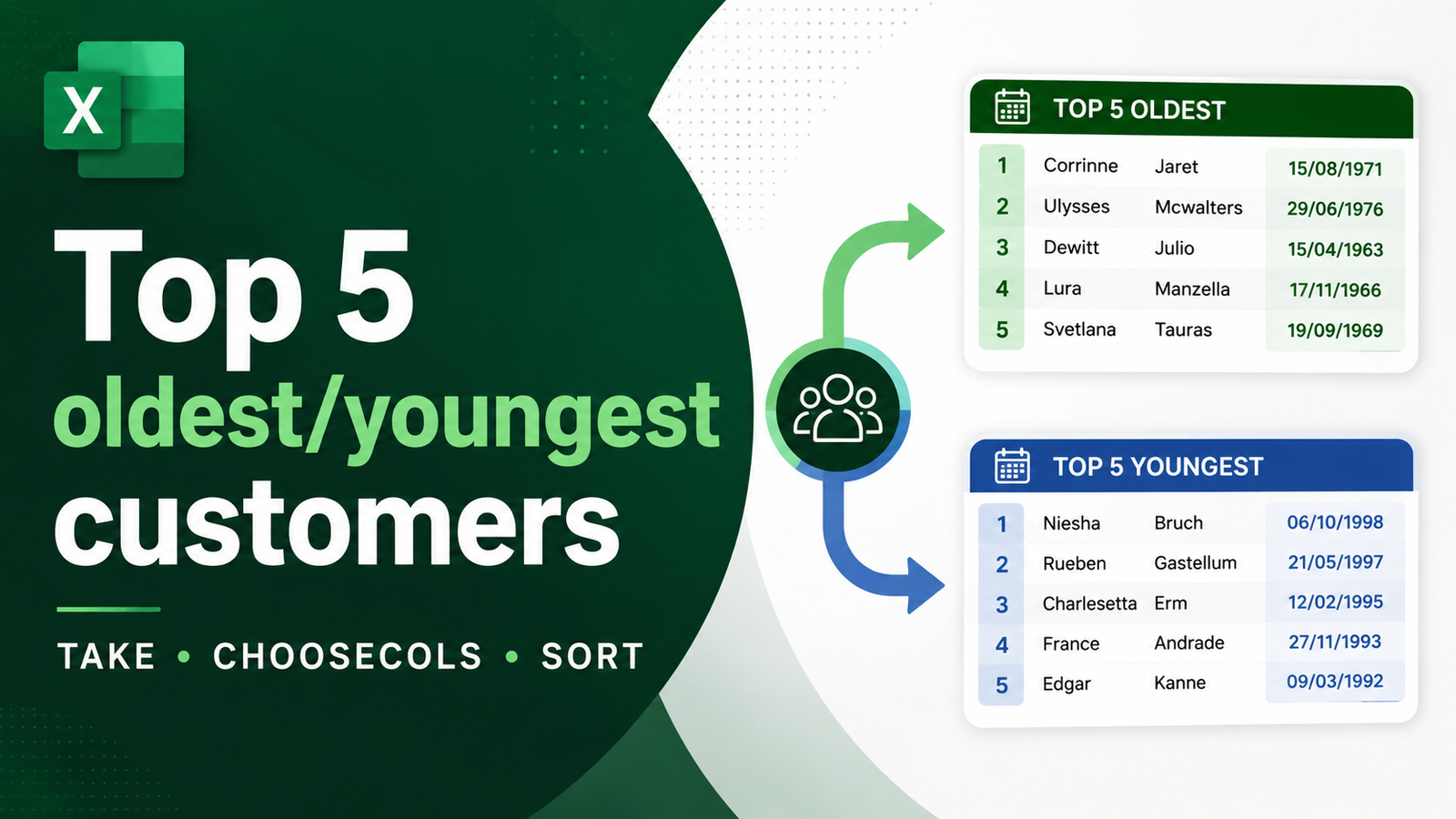
Top 5 Oldest/Youngest Customers
Filtering and sorting a dataset allows you to analyse it more effectively by hiding the surplus and putting column data in ascending or descending order.
An Excel Table provides the tools to do this; however, clearing the filter and sort state means your results are lost, so you may want something more permanent.
Formulas give you the flexibility to decide what, where, and how the data gets outputted.
Recently, Microsoft announced several new functions, including TAKE and CHOOSECOLS. Both are currently only available to Office Insiders on the Beta Channel.
New Functions
- TAKE — returns rows or columns from the start or end of an array.
= TAKE ( array , rows, [columns] )- CHOOSECOLS — returns specific columns from an array.
= CHOOSECOLS ( array , col_num1 , [col_num2] , … )Example
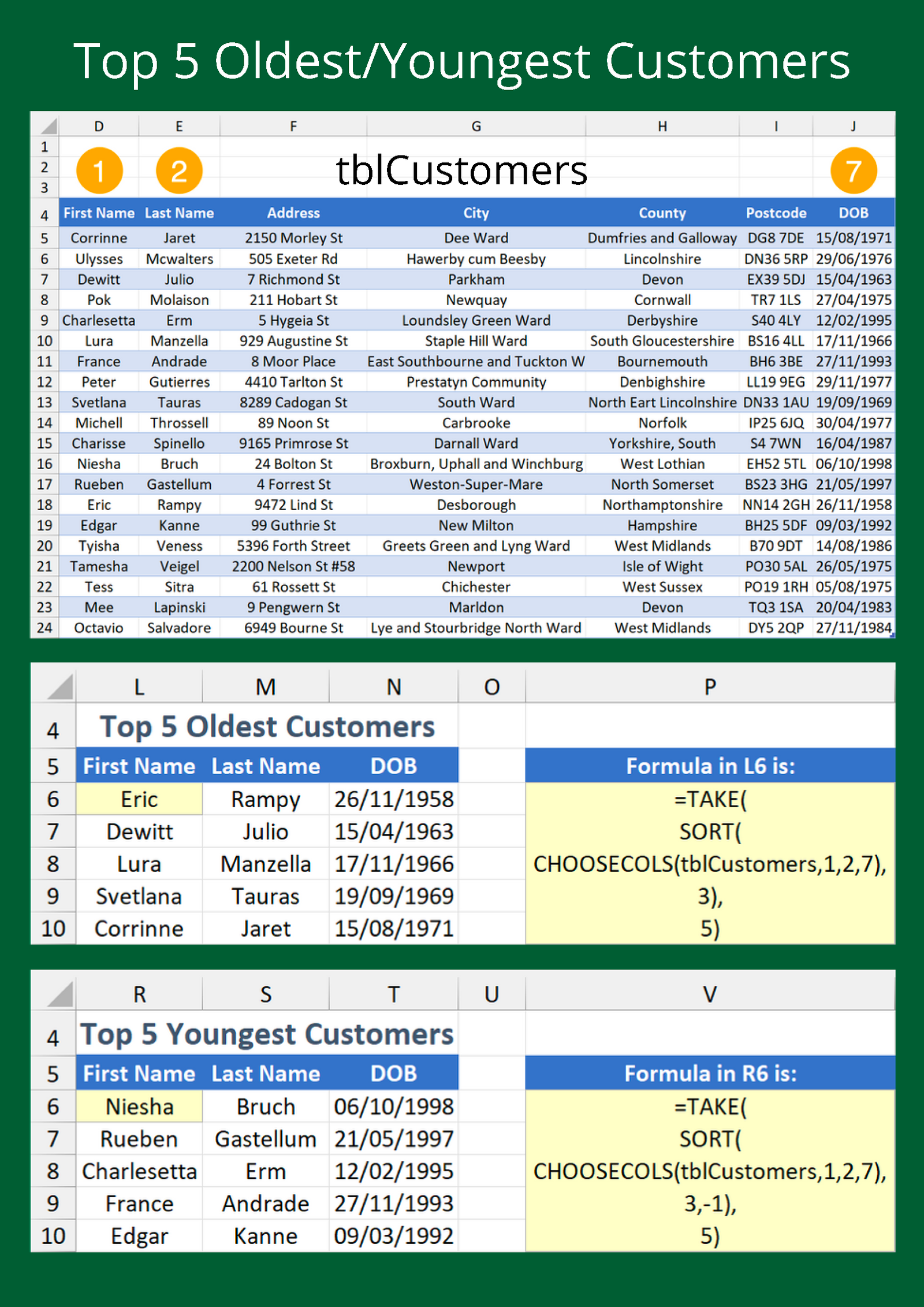
A table called tblCustomers contains the customer data from which to return the five oldest and youngest customers. Moreover, we are only interested in the First Name, Last Name and DOB columns.
This is where CHOOSECOL comes in handy, as tblCustomers occupies the array argument and each column number is housed in col_num1, [col_num2] and [col_num3], respectively.
SORT’s [sort_index] contains 3 to sort by the third column (DOB) of the new array. As it arranges in ascending order by default, [sort_order] is omitted for finding the oldest customers, but -1 is necessary for the youngest.
At this stage, the results are sorted but all 20 rows display. Wrap TAKE around the SORT statement and include 5 in rows to only return the top five.


