BYCOL Function

The new BYCOL function is currently only available to Office Insiders, but it promises to make calculating columns easier and more efficient.
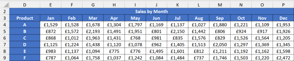
The Sales by Month table contains monthly sales figures for six products.
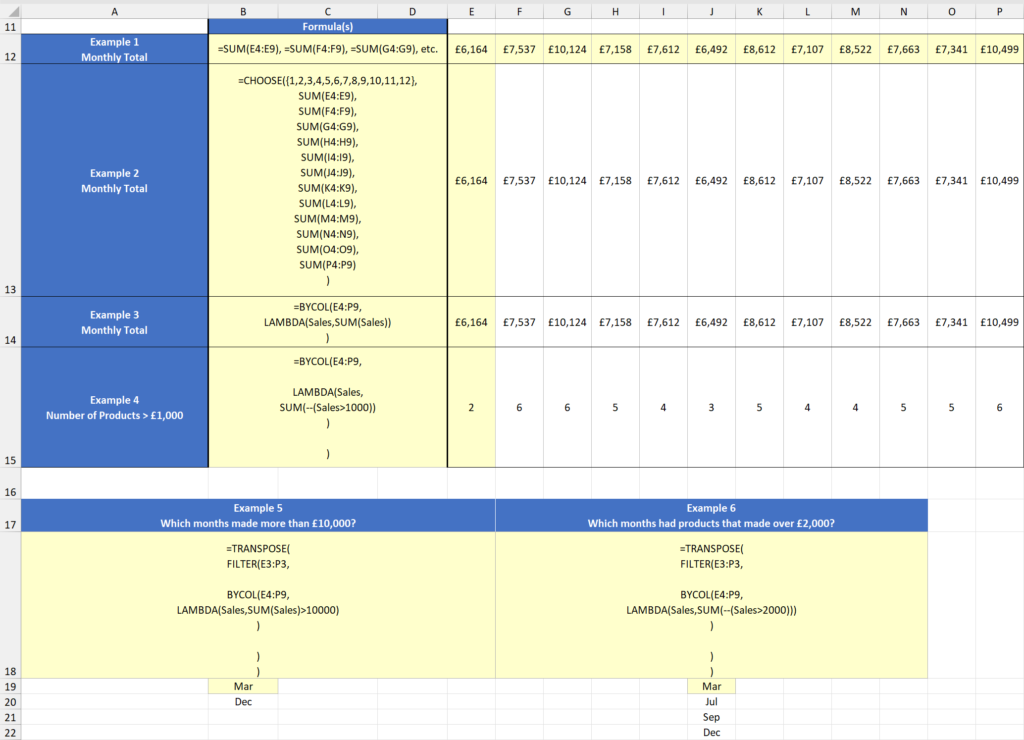
If you wanted to calculate the total for each month, you’d likely use 12 SUM formulas (Example 1). This works as far as results, but it’s based on a decentralised approach.
Example 2 offers an alternative, which uses the CHOOSE function to group the SUM statements in a single formula, spilling them across the adjoining cells. This is better, as it reduces the risk of issues later on, however, it is rather lengthy.
Example 3 introduces BYCOL to carry out the same task — with a much shorter formula.
The syntax is:
BYCOL (array, [function])array— the array to break down by column.[function]— a LAMBDA to apply on each column.
The formula starts with BYCOL and references the sales figures in its array argument. In [function], LAMBDA holds a parameter named Sales, which is used in the SUM calculation. Each column of the sales table is totalled up to return 12 separate results.
Example 4 returns the number of products for each month that made more than £1,000. The previous LAMBDA calculation is altered to become SUM(--(Sales>1000)), which generates an array of TRUE/FALSE values that coerce into 1s and 0s, allowing the SUM function to add them up.
Example 5 asks the question: which months made more than £10,000?
This time the calculation is SUM(Sales)>10000). The whole BYCOL statement is nested in FILTER’s include argument, with the months referenced in array. The ones that made more than £10,000 are returned, but instead of spilling horizontally, TRANSPOSE flips them around to display vertically.
Finally, Example 6 uses a similar formula to list the months that had products generating over £2,000.


