Combining Multiple Excel Tables Into One
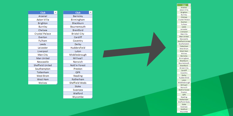
A few months ago I encountered a scenario I hadn’t faced before. I was dealing with a large number of financial transactions from multiple bank accounts that were being housed in separate Excel worksheets. I needed to consolidate them so they would appear in one single table. This was part of an interactive profit and loss system I was building.
It may sound like a simple task, but I needed an automated solution that would update in real time.
Like with any Excel conundrum you’re faced with, the first port of call is trusty Google. Surprisingly though, after scouring the internet for hours, I found it was bereft of solutions.
What didn’t help was I had to think about compatibility because the version of Excel the company was using was Excel 2016 for macOS. This was hardly ideal — because as many of you may already know — it is a shadow of the Windows equivalent. I like to keep up to date with the very latest version myself, which is why Microsoft 365 (formerly Office 365) for Windows is the best one to have.
After digging and poking around, I uncovered several different techniques. I’m going to show you five methods you can use in Excel to combine multiple tables. They each have pros and cons, but hopefully they will help you in the future if you are faced with a scenario that requires them.
Download Examples
Download link: Combining-Lists.xlsx
⚠️ Quick caveat: an up-to-date Microsoft 365 desktop copy of Excel is recommended, as some of the methods will not work on previous versions. However, feel free to use your old copy—just don’t complain when you find some of the methods aren’t working.
Workbook
You will see there are three tables containing English football clubs:
- Table A — Premier League clubs
- Table B — Championship clubs
- Table C — League One clubs
To combine them, the following methods can be used:
Method 1
Let’s use cell G6 as an example:
=INDEX(

IF(
ROWS(G$6:G6)
<=
ROWS(TableA[Club]),

TableA[Club],TableB[Club]),

IF(ROWS(G$6:G6)
<=
ROWS(TableA[Club]),

ROWS(G$6:G6),
ROWS(G$6:G6)-ROWS(TableA[Club]))

)
This formula is based on the INDEX function. The array argument’s purpose is to determine whether Table A or Table B should be outputted. It consists of an IF statement that checks if the number of rows in range G$6:G6 is less than or equal to the amount in Table A (1<=20). If this logical_test equates to true (in this case it is), then output the values from Table A —or if false—from Table B.
As the row number in the second part of the G$6:G6 range is relative, it will change incrementally as the formula is populated downwards.
The cut-off point is cell G26, as this is where the values of Table B begin. Here, the logical_test converts to 21<=20, which triggers the false argument, so Table B’s values are outputted.
The second INDEX argument is row_num, and this is responsible for the row number that holds the club that’s outputted from array.
IF(ROWS(G$6:G6)<=ROWS(TableA[Club]),
ROWS(G$6:G6),
ROWS(G$6:G6)-ROWS(TableA[Club])
)
Similarly to array, the same IF condition is present for logical_test, but the value_if_true argument equals true as long as there are still clubs in Table 1 to be displayed. However, if there are not, then it jumps to value_if_false, which takes away the number of rows in Table A (20) from the ROWS(G$6:G6) dynamic reference (1 and counting).
If you select an argument and press F9, you can convert it into a value. Do this for each one and it’ll make it clearer what is happening:
IF(1<=20,1,1–20))Cell G25 returns Wolves and is the last formula in this sequence to equal true.
IF(20<=20,20,20–20))G26 contains Barnsley, which is the first entry of Table B. As the condition 21<=20 is false, the sum 21 minus 20 is calculated, meaning 1 is the row number.
IF(21<=20,21,21-20))You can see how the array and row_num arguments of INDEX work in tandem. Given they both use the same logical condition, they will always be either true or false simultaneously.
It’s worth noting that this formula will only work when you have two tables you want to combine. The main advantage though is compatibility, as it will work with Excel 2007 onwards.
Method 2
This technique uses some of the same principles as Method 1, but with a few notable differences.
Let’s look at cell I6:
=IFERROR(
INDEX(
OFFSET(A$6,0,0,SUMPRODUCT(--(LEN(TableA[Club])>0))),
ROWS($I$6:$I6)),

IFERROR(
INDEX(
OFFSET(C$6,0,0,SUMPRODUCT(--(LEN(TableB[Club])>0))),
ROWS($I$6:$I6)-SUMPRODUCT(--(LEN(TableA[Club])>0))),
"")
)
The formula starts off with the IFERROR function and is broken down into two parts: value represents Table A and value_if_error Table B.
Just like with Method 1, INDEX allows for an array and row number to be calculated to retrieve the correct value.
In the array argument, the OFFSET function references A$6 as the starting point, and as there is no need to deviate from this position, 0 is given for the rows and cols arguments.
The role of height is to find the number of cells in Table A that are not blank, and then change the scope of the reference to satisfy that condition. Whilst A$6 was set as the initial cell, the range becomes A$6:A25 to cover all the clubs in the table.
OFFSET(A$6,0,0,SUMPRODUCT(--(LEN(TableA[Club])>0)))The LEN function on its own returns the character length of a cell. So it looks at each value in Table A and checks it is greater than 0.
--(LEN(TableA[Club])>0) = {1;1;1;1;1;1;1;1;1;1;1;1;1;1;1;1;1;1;1;1}
The -- is used to coerce TRUE and FALSE values into binary figures. Without it, it would read as: {TRUE;TRUE;TRUE;TRUE;TRUE;TRUE;TRUE;TRUE;TRUE;TRUE;TRUE;TRUE;TRUE;TRUE;TRUE;TRUE;TRUE;TRUE;TRUE;TRUE}.
This is necessary so that when the SUMPRODUCT function is wrapped around it, each chunk of the array is added up to produce the value 20.
A height of 20 means that the initial starting point of A$6 becomes a range that extends 20 rows down: A$6:A25.
The final argument is row_num, and ROWS($I$6:$I6) ensures the row number increases incrementally by one to output all the clubs in the array.
If the value argument produces a #REF! error, it means that the row_num value exceeds the number of rows in Table A, so value_if_error is proceeded with for Table B.
IFERROR(
INDEX(
OFFSET(C$6,0,0,SUMPRODUCT(--(LEN(TableB[Club])>0))),
ROWS($I$6:$I6)-SUMPRODUCT(--(LEN(TableA[Club])>0))),
"")
This part is largely the same as value, but because a second table is being added, a modification must be made to the row_num argument of INDEX.
Instead of only using ROWS($I$6:$I6), the additional part SUMPRODUCT( — (LEN(TableA[Club])>0)) is subtracted from it. This ensures the row number produced will be viable for extracting values from Table B. For cell I6, -19 is returned, but that doesn’t matter because this part of the formula is ignored anyway until all the values from Table A have been returned. In I26—where the first value of Table B is displayed—it’s 1.
This method—unlike Method 1—does allow for more than two tables to be combined. In column J, you will see an example with three tables stacked.
The process is quite straightforward. You only have to copy the previous part of the formula and edit the INDEX array to include Table C instead. Then put -SUMPRODUCT( — (LEN(TableB[Club])>0)) at the end of the row_num argument to subtract the rows of Table B.
IFERROR(
INDEX(
OFFSET(E$6,0,0,SUMPRODUCT(--(LEN(TableC[Club])>0))),
ROWS($J$6:$J50)
-
SUMPRODUCT(--(LEN(TableA[Club])>0))
-
SUMPRODUCT(--(LEN(TableB[Club])>0))),
"")
In cell J50, look at what is taking place…
ROWS($J$6:$J50)-SUMPRODUCT(--(LEN(TableA[Club])>0))-SUMPRODUCT( — (LEN(TableB[Club])>0)) converted into values is: 45–20–24, which equals 1.
Like Method 1, this is also good to use when compatibility is of concern. Be aware though that the OFFSET function is volatile, meaning any cell that contains this function will recalculate whenever Excel processes a change in the workbook. This can slow things down if you have a large amount of data.
Method 3
This method utilises Excel’s dynamic array capabilities so you will need to have Microsoft 365 for it to work.
=IFERROR(INDEX(TableA[Club],
SEQUENCE(ROWS(TableA[Club])+ROWS(TableB[Club]))),
INDEX(TableB[Club],
SEQUENCE(ROWS(TableA[Club])+ROWS(TableB[Club]))
-
ROWS(TableA[Club]))
)
It is based on the IFERROR function and broken down into two parts again. The value argument contains instructions for extracting the clubs from Table A, whilst value_if_error does the same for Table B.
Similarly to the two previous methods, INDEX holds the array and defines the row number. The key difference is that relative cell references have been neglected in favour of structured references.
Wrapping the SEQUENCE function around the two ROWS statements creates an array of 44 sequential numbers, adding up to the total number of clubs there are.
SEQUENCE(
ROWS(TableA[Club])
+
ROWS(TableB[Club])
)
You must remember that this is a dynamic array formula, so it only exists in one cell. Every value you see sprawled downwards originates from the formula in cell L6.
Once you’ve understood this concept, you’ll realise that when the row number exceeds the number of clubs in Table A, an error will be produced, triggering the value_if_error argument to be evaluated.
INDEX(

{“Arsenal”;”Aston Villa”;”Brighton”;”Burnley”;”Chelsea”;”Crystal Palace”;”Everton”;”Fulham”;”Leeds”;”Leicester”;”Liverpool”;”Man City”;”Man United”;”Newcastle”;”Sheffield United”;”Southampton”;”Tottenham”;”West Brom”;”West Ham”;”Wolves”},
 {1;2;3;4;5;6;7;8;9;10;11;12;13;14;15;16;17;18;19;20;21;22;23;24;25;26;27;28;29;30;31;32;33;34;35;36;37;38;39;40;41;42;43;44}

)
The second half of the formula belongs to Table B and is much the same as the first, except -ROWS(TableA[Club]) is added to the end to subtract the 20 rows in Table A.
SEQUENCE(ROWS(TableA[Club])+ROWS(TableB[Club]))-ROWS(TableA[Club]
= SEQUENCE(20)+24)-20
INDEX(
  {“Barnsley”;”Birmingham”;”Blackburn”;”Bournemouth”;”Brentford”;”Bristol City”;”Cardiff”;”Coventry”;”Derby”;”Huddersfield”;”Luton”;”Middlesbrough”;”Millwall”;”Norwich”;”Nott’m Forest”;”Preston”;”QPR”;”Reading”;”Rotherham”;”Sheffield Weds”;”Stoke”;”Swansea”;”Watford”;”Wycombe”},
  {-19;-18;-17;-16;-15;-14;-13;-12;-11;-10;-9;-8;-7;-6;-5;-4;-3;-2;-1;0;1;2;3;4;5;6;7;8;9;10;11;12;13;14;15;16;17;18;19;20;21;22;23;24}

)
You may be wondering why ROWS(TableA[Club] has been added and then taken away. Because this part of the formula will not be evaluated until all the values from Table A have been displayed, it is necessary to create a 44 value array where the first 20 comprises minus figures and a 0. Whilst these are not responsible for output themselves, they are imperative because they act as placeholders for Table A’s values and allow the 21st value (start of Table B) to be shown in the correct cell.
{-19;-18;-17;-16;-15;-14;-13;-12;-11;-10;-9;-8;-7;-6;-5;-4;-3;-2;-1;0;1;2;3;4;5;6;7;8;9;10;11;12;13;14;15;16;17;18;19;20;21;22;23;24}Notice how the subtraction of ROWS(TableA[Club] occurs outside the SEQUENCE function and not in it. This is a clever trick to prevent the first 20 array values from being positive numbers. It’s not possible to have non-positive row numbers, but as soon as they become positive, they are being read.
Without ROWS(TableA[Club] being subtracted, the following would result:
{1;2;3;4;5;6;7;8;9;10;11;12;13;14;15;16;17;18;19;20;21;22;23;24;25;26;27;28;29;30;31;32;33;34;35;36;37;38;39;40;41;42;43;44}Only the last four clubs from Table B would be outputted: Stoke, Swansea, Watford and Wycombe. Their row numbers happen to be 21, 22, 23 and 24 respectively. The 20 other cells would all have #REF! errors because there are not more than 24 rows in Table B.
Note that this method only allows for two tables to be combined.
Method 4
I’ll start by saying there’s a good chance you’ve never come across the FILTERXML function before, so it’s worth exploring its uses beyond what I’m going to show you.
XML is a mark-up language designed to store and transport data. It consists of a collection of custom tags, which are not predefined like with HTML, and the structure is flexible. Whereas HTML is a presentation language, XML is a data-description language used by a variety of applications to output data.
The purpose of this function is to return specific data from XML content by using a defined XPath. XPath is the query language used to select nodes from an XML document.
Let’s home in on cell N6:
=FILTERXML("<table><team>"&TEXTJOIN("</team><team>",,TableA[Club],TableB[Club])&"</team></table>","//team")The first argument is xml, where a string in XML format is stated. Remember, the tags you see are custom—they can be named anything, but as they come in pairs, there must be a starting and closing one for each.
=FILTERXML("<table><club>"&TEXTJOIN("</club><club>",,TableA[Club],TableB[Club])&"</club></table>","//club")I’ve used the strings "<table><club>" and "</club></table>" at opposite ends to sandwich in the values of Table A and Table B. This is done with the help of the TEXTJOIN function, where the delimiter "</club><club>" is set so these tags surround each club.
TEXTJOIN("</club><club>",,TableA[Club],TableB[Club])One of the best things about this method is how easy it is to combine additional tables. It is a simple case of adding a range to another text argument. A maximum of 252 are permissible.
The xpath argument defines the node to be selected. Many path expressions exist, but using // selects all nodes that match a certain name. So by putting "//club", the <club> element will be targeted. You could also use "/table/club" and the same result would occur, as a single / selects from the root node.
If you wanted to target the fifth row number of the list, for instance, "//club[5]" would result in only Chelsea being outputted.
It’s worth checking out w3schools for more details about the different XPath expressions you can use.
Another useful thing to know is that this is the only method that ignores empty cells if they exist mid-way through a table. All the others will display a 0 for blank values.
Method 5
This final method is not a formulaic solution, but it utilises Power Query instead. It’s the easiest way of combining two or more tables, but has the downside of not updating instantly like formulas do.
You may not be familiar with what Power Query is, but in simple terms it is a data cleaning, transformation and preparation tool that has an engine of its own. There are many tasks that can be carried out in regular Excel using formulas. However, Power Query has a useful interface containing many features that can be applied without any formula knowledge, often saving you time. Aside from combining tables, examples include adding conditional columns, stripping whitespaces, replacing values and extracting characters.
With no formulas to dissect, let’s look at the stages involved to combine Table A and Table B.
For Power Query to interact with Excel tables, they must first be loaded into the engine. This has to be done one at a time.
Make sure the active cell is anywhere inside Table A and then go to the Data tab to find the From Table/Range button in the Get & Transform Data section.

Clicking on that brings up the Power Query Editor window.
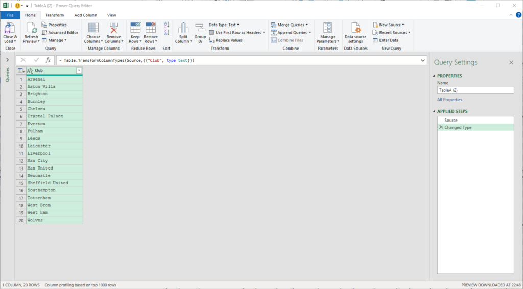
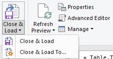
On the far left, go to the Close & Load dropdown and click on Close & Load To… button.
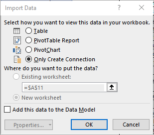
Choose Only Create Connection, as this data only needs to be brought into Power Query. Then click OK.
In the side panel on the right, the connection to Table A will appear under the Queries tab.
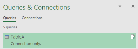
The same process is carried out for Table B…
Now there are two tables in the panel, right-click on Table A and select Append.
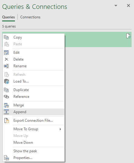
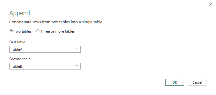
The Append window pops up and allows you to choose between appending two tables, or three or more. The default option is Two tables, so I will keep it selected for this example.
For the First table dropdown, Table A is the base table so will already be present, hence you need to select Table B in the Second table dropdown.
Click OK.
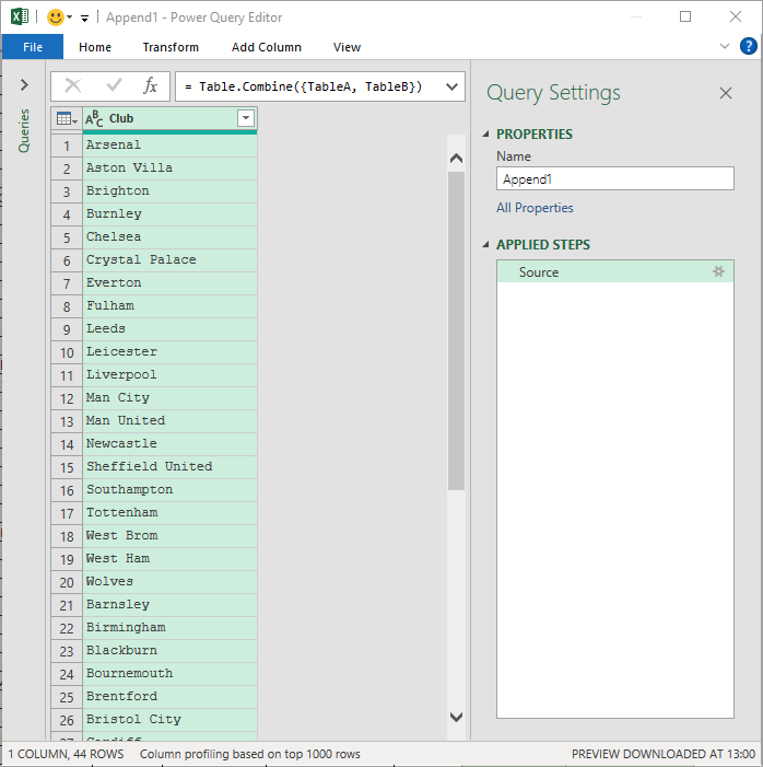
This brings up the Power Query Editor window again, which contains the appended table.
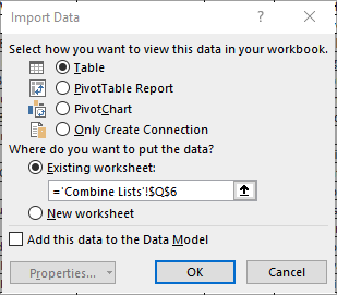
The last step is to publish the table to the worksheet. Click on the Close & Load To option again from the dropdown, and then choose Existing worksheet to decide where the table should be placed.
Click OK.
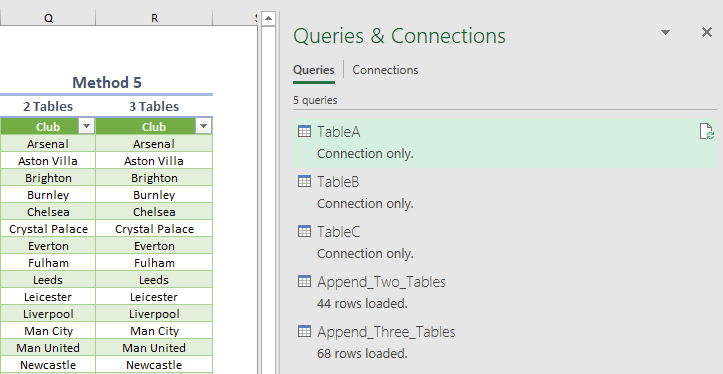
Voila! The appended table is loaded into the worksheet and listed in the side panel. If you right-click it and select Rename, you can name it what you like to help distinguish between different queries.
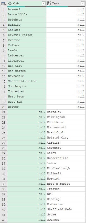
One final thing I’ll say is that it’s important to ensure the tables being appended have the same column names, otherwise Power Query will output them in separate columns.
Conclusion
There are pros and cons of each method. The decision about which one to use comes down to your requirements. If you have Microsoft 365 for Windows and you’re working on a workbook no one else will use — then great. You haven’t really got to worry about anything.
However, in the workplace you potentially have to think about the Excel version the company uses, hardware considerations and your colleagues’ knowledge of Excel. Furthermore, how many tables do you want to combine?
My advice for most people is that Method 5 is the best option providing you have Power Query in your version of Excel. If you’ve got Excel 2010/2013, Power Query is available as an add-in, although it’s no longer updated by Microsoft.
If compatibility is of the utmost importance, then use Method 1 or Method 2, although be aware that Method 1 can only combine two tables.
Method 3 and Method 4 both utilise Excel’s dynamic array capabilities, so you’ll need Microsoft 365 for these. Once you’ve got to grips with the basics of XML, you’ll realise how great Method 4 is. It is the shortest formulaic solution and has the advantage of ignoring blank values, which none of the others do.
Stacking separate tables shouldn’t be this difficult though. I really hope Microsoft make a function available in due course that allows us to do it with ease. Maybe not even a function—something like ={TableA;TableB;TableC} would suffice. Dynamic array capabilities have certainly given me hope that it won’t be too far away.
Functions Used
FILTERXML
INDEX
IF
IFERROR
LEN
OFFSET
ROWS
SEQUENCE
SUMPRODUCT
TEXTJOIN