
When to use FILTER over XLOOKUP in Excel


There are numerous ways to find the highest value in a column and return one or more values in the matching row.
In this example, a table called tblSales houses some monthly sales data.
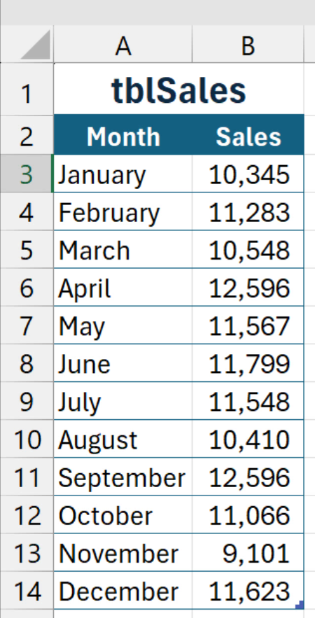
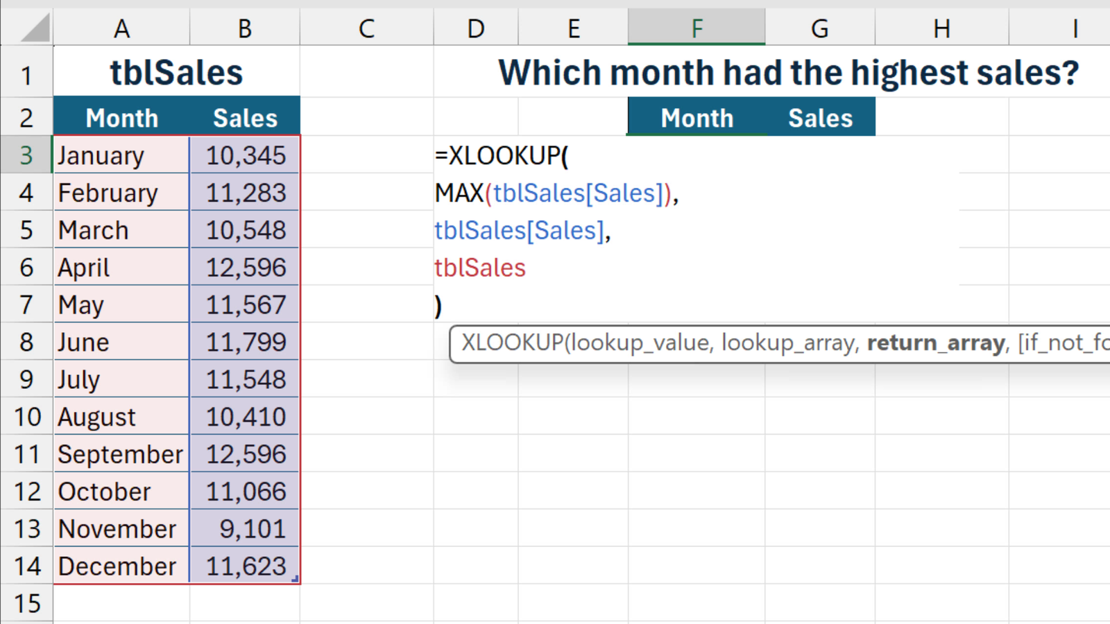
XLOOKUP is combined with MAX to find the maximum figure in the Sales column and return that and the adjacent month.
=XLOOKUP(
MAX(tblSales[Sales]),
tblSales[Sales],
tblSales
)
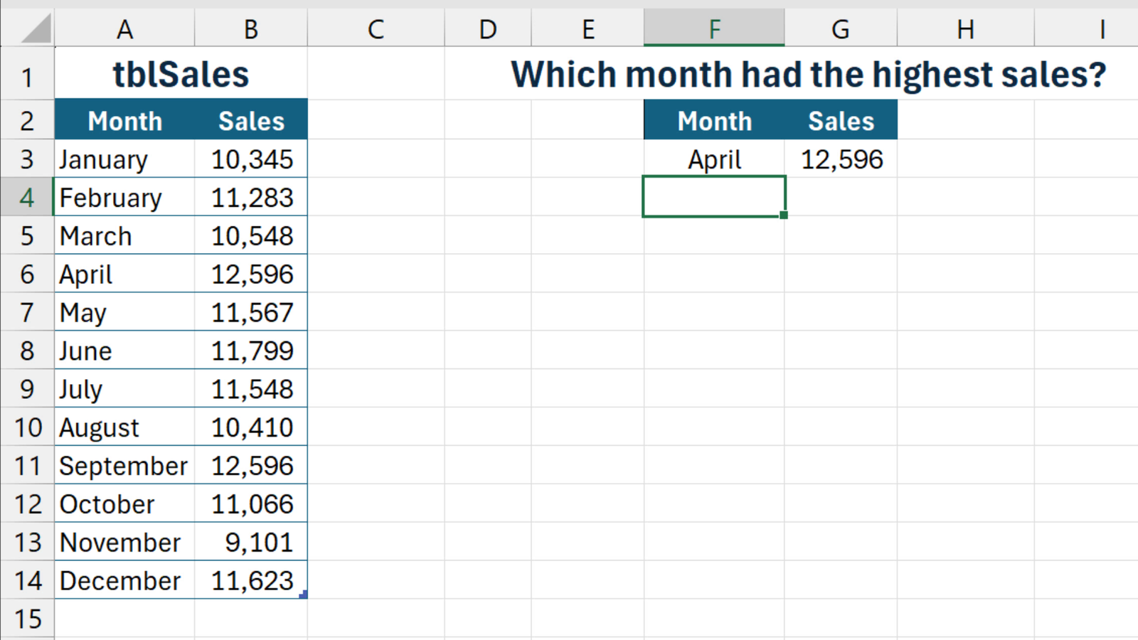
This works — sort of. It’s best when there are no duplicates, as only the first matching row is considered. In this case, April and 12,596 are returned, whereas September is ignored.
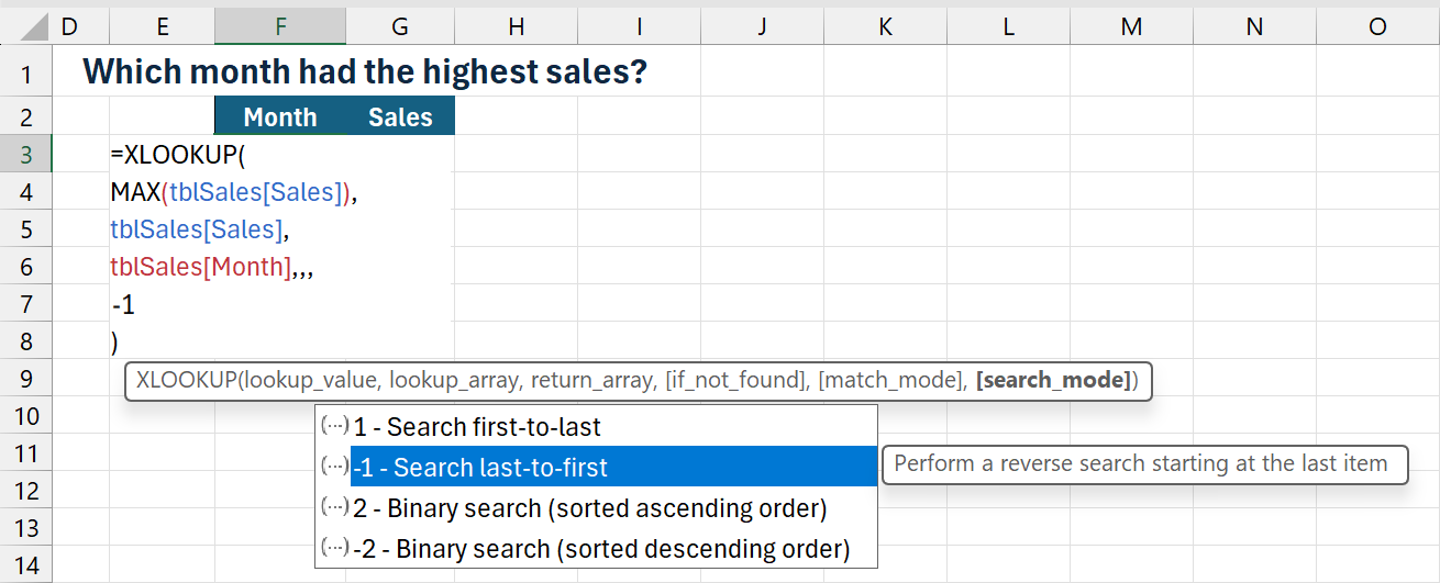
You could set the [search_mode] to -1 so the lookup starts from the bottom, meaning September would take precedence.
However, the benefit of using FILTER is that it returns both April and September, as the function is designed to handle multiple results.
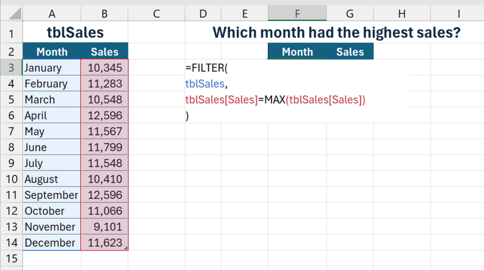
=FILTER(
tblSales,
tblSales[Sales]=MAX(tblSales[Sales])
)
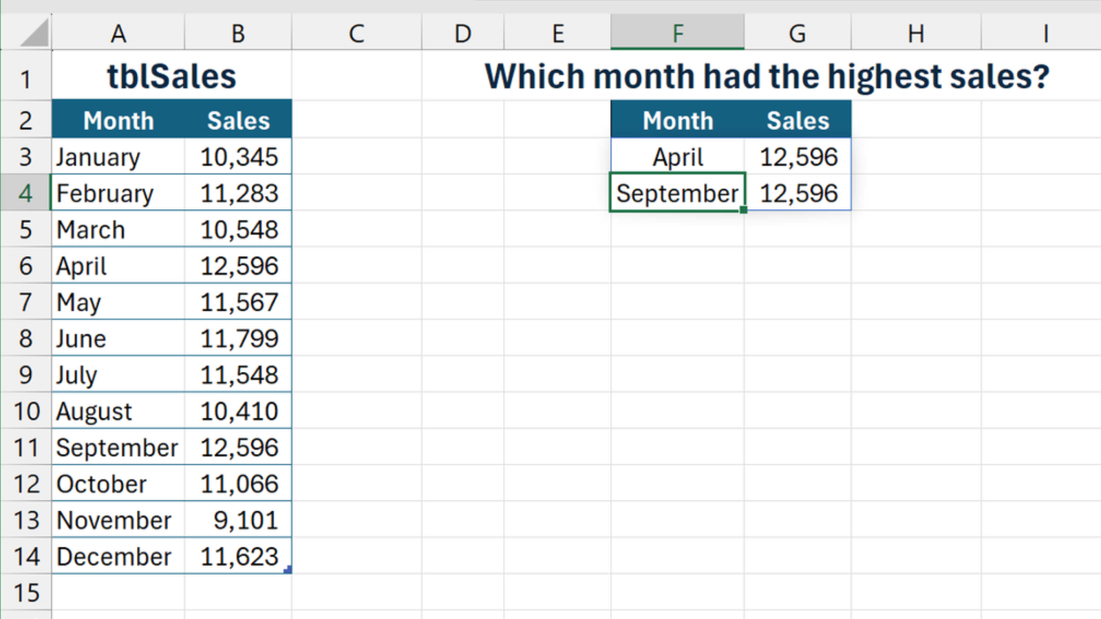
The takeaway is to always be aware of this type of scenario, so you use the right function for your needs.