The Ultimate Guide to Excel Tables
A table is defined as “a set of facts or figures systematically displayed, especially in columns.” They structure data in a way that ensures fast and efficient readability.
In Excel, they have official status. A table is an object with its own features and capabilities.
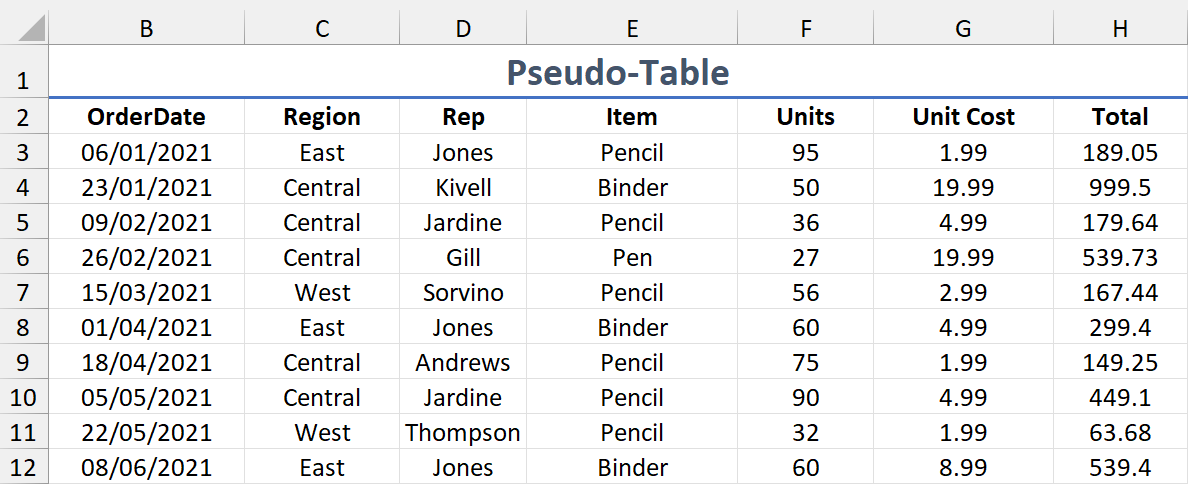
Simply dumping some data onto a worksheet and applying colour and border formatting is nothing more than a facade. Pseudo-tables do not give you any functional advantages.
Real tables can filter and sort data, expand and shrink, as well as use structured references.
They first appeared in Excel 2007, although in prior versions were called lists and offered the same basic features.
This article explores the ins and outs of tables and how to use them effectively.
CONTENTS

· Table Parts
  ∘ Header Row
  ∘ Data
  ∘ Row
  ∘ Column
  ∘ Total Row
· How to Create a Table
  ∘ From the Ribbon
  ∘ Keyboard Shortcut
· Table Design Contextual Tab
· Hide the Header Row
· Show the Total Row
· Emphasise First and/or Last Column
· Banded Rows and Columns
· Sort and Filter
· Table Names
  ∘ Table Name Rules
  ∘ Header Name Rules
· Select a Table in the Name Box
· Resize the Table
  ∘ From the Ribbon
  ∘ With the Resize Handle
· Tables Expand Automatically
· Insert Rows or Columns
· Delete Rows or Columns
· Select Table Parts
  ∘ Select a Column
  ∘ Select a Row
  ∘ Select the Data
  ∘ Select the Header Row
  ∘ Select the Total Row
· Move a Table
· Summarize with PivotTable
· Remove Duplicate Values
· Convert a Table to a Range
· Insert a Slicer
· Customise the Table Style
  ∘ Custom Table Styles
· Structured Referencing
· Structured Reference Examples
  ∘ Examples of Active Row Structured References
  ∘ Examples of Data Structured References
  ∘ Examples of Column Structured References
  ∘ Examples of Header Structured References
  ∘ Examples of Total Structured References
· Pseudo-Table and Table Tests
  ∘ Delete Rows 6 to 9
  ∘ Insert 4 Rows Below Row 5
  ∘ Add a New Value to the Rep Column
  ∘ General Remarks
· Calculated Columns
  ∘ Turn Off Calculated Columns
· Column Headers Stay Visible
· Referencing Using AutoComplete
· Summary
Table Parts
Every table is composed of the same parts, and it’s worth getting familiar with these as they will be referred to throughout the article.
Header Row
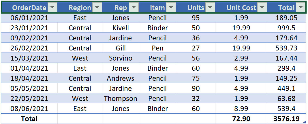
The top row of a table contains the column names, which must be unique text values. Formulas are prohibited.
Data
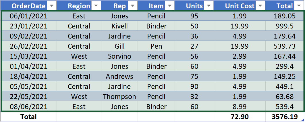
The cells containing the values and formulas are collectively called the data.
Row
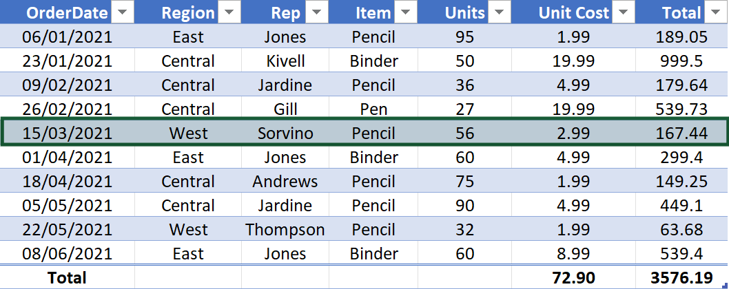
A row is a single set of horizontal data cells. Any table must have at least one row so attempting to delete all of them will always leave a sole survivor.
Column
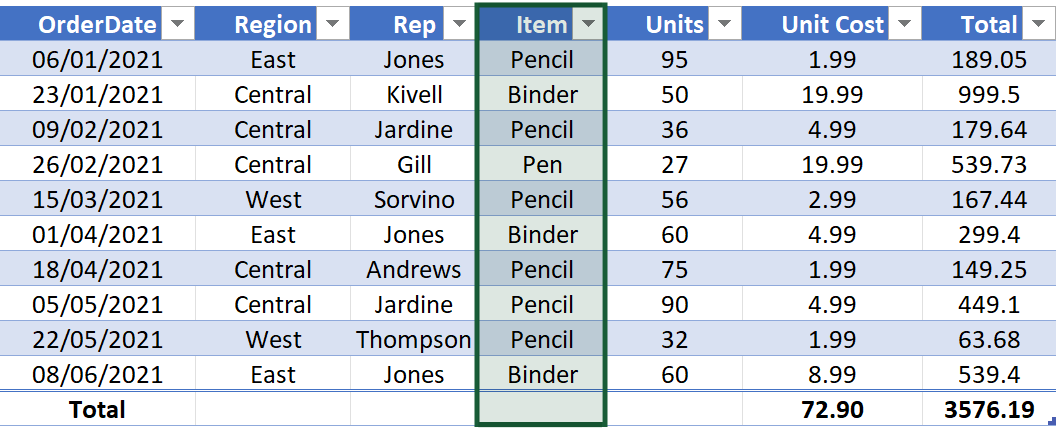
A column is a single set of vertical cells. Any table must contain at least one column; however, unlike rows, deleting all of them also removes the whole table.
Total Row
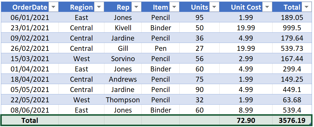
The Total Row calculates column data, such as the sum, count or average.
How to Create a Table
From the Ribbon
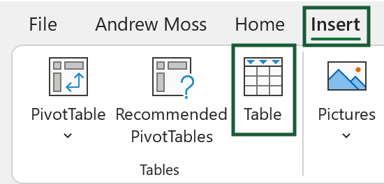
Activate any cell in your data and select Insert (tab) > Table (button).
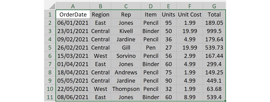
Excel will intelligently set the boundaries of where it thinks your table is by wrapping a dotted line around it. If this range is wrong, you can manually adjust it in the Create Table pop-up window.

Ensure your data is surrounded by a perimeter of empty cells (excluding the sides adjacent to the row and column headings). Otherwise, the non-empty ones will be mistaken as being part of the range.
To avoid any guesswork, another way is to select the exact range of your data and then click the Table button.
If your data’s column headers are in the first row, tick the My table has headers checkbox and then click OK.
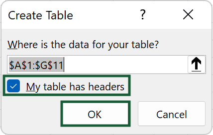
This will make the first row column headers.

Leaving it unchecked will add a row of generic column headers to the top of your data, e.g. Column1, Column2 and Column3.

Keyboard Shortcut
As an alternative to the ribbon button, press Ctrl + T (or Ctrl + L) to bring up the Create Table window.
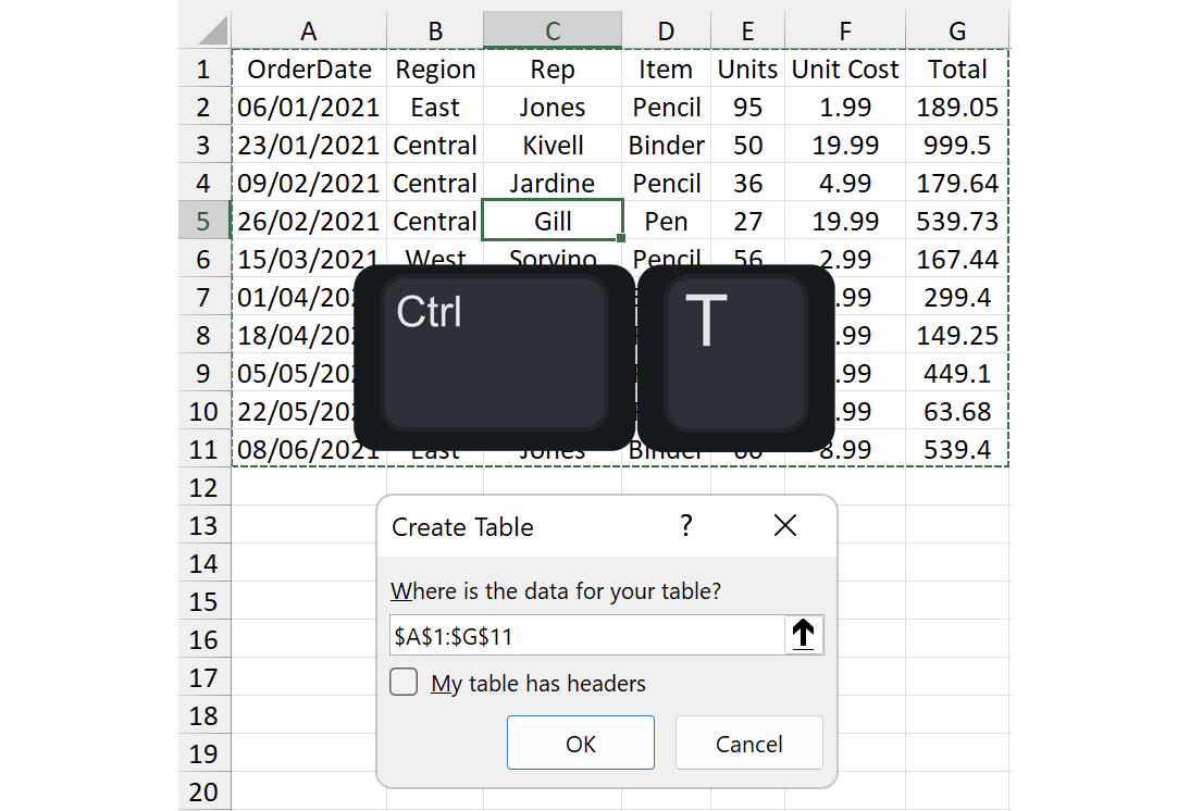
Table Design Contextual Tab
Selecting any cell in a table will activate the Table Design contextual tab in the ribbon.

This houses all the table’s properties, tools, and styling options.
It will disappear when the active cell does not belong to a table.
Hide the Header Row
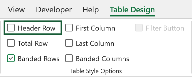
To hide the column names, turn off the Header Row checkbox. This will also disable the Filter Button.

Show the Total Row
By default, the total row does not display but can be enabled by ticking the Total Row checkbox on the Table Design contextual tab.

When you first add the Total row to a table, ‘Total’ appears in the leftmost column and either a sum or count in the rightmost (depending on the values detected).
Each cell in the total row has a dropdown that contains a choice of aggregation types. These generate formulas that perform calculations on the column. They are all based on the versatile SUBTOTAL function, which effectively has numerous sub-functions built into it.
For example, =SUBTOTAL(109,[Total]) calculates the sum of the Total column. The function_num is 109, meaning hidden rows will not be included in the calculation. The same applies to the others.
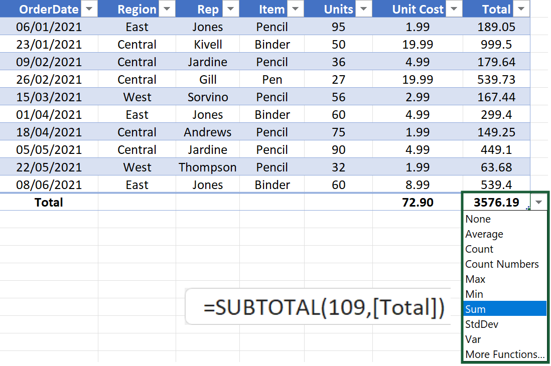
If the default choices don’t suffice, you are also allowed to use your own formulas.
Emphasise First and/or Last Column
If the first and last columns are particularly significant, you may want them to stand out.
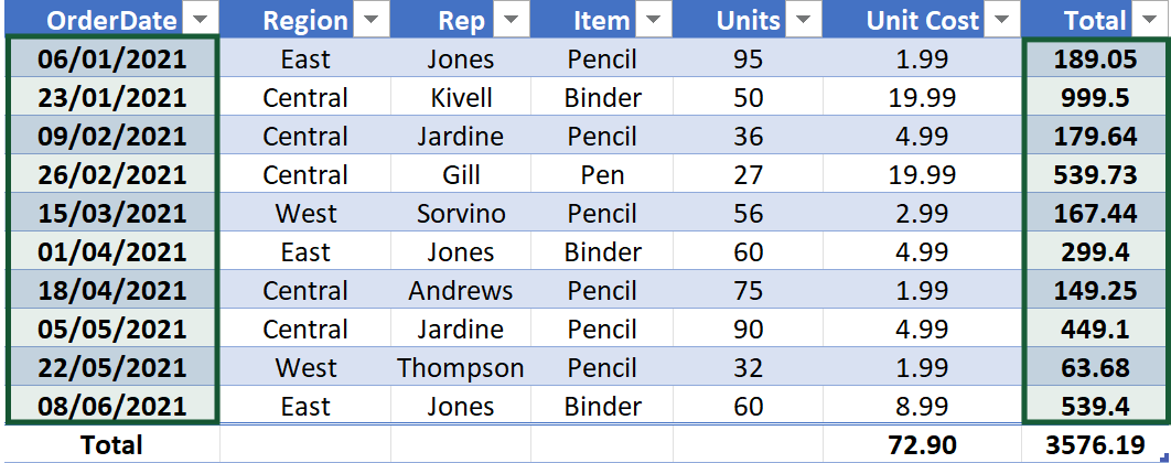
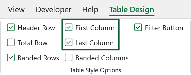
Tick the First Column and/or Last Column checkbox(es) to apply bold formatting to the data.
Banded Rows and Columns
Colouring table rows and columns in alternating shades can serve as a visual aid. Any new table will have banded rows by default, but you can toggle this and banded columns on or off to suit your needs.
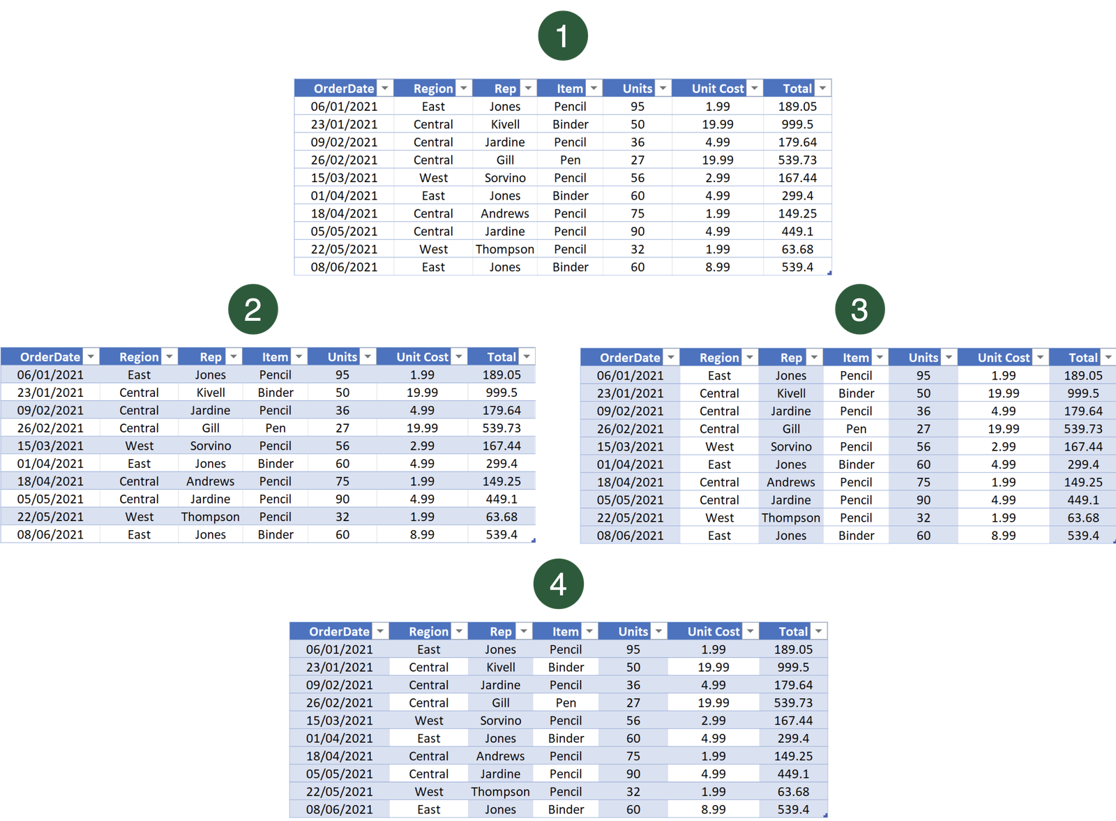
- No banding
- Banded rows only
- Banded columns
- Banded rows and columns
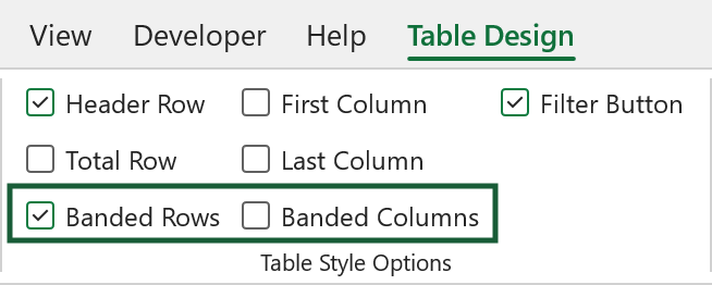
The Banded Rows and Banded Columns checkboxes are found on the Table Design contextual tab in the Table Style Options group.
Sort and Filter
A dropdown button is automatically added to each column header of a new table. It allows you to access and apply the sort and filter options.
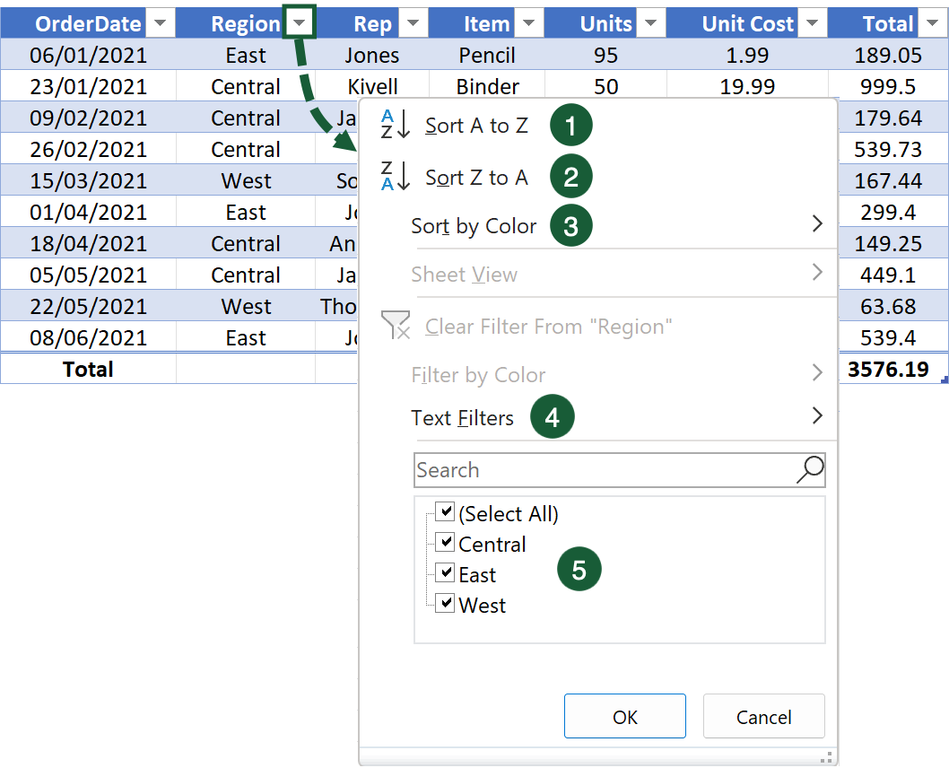
Here are a few of the options you might use:
- Sort A to Z sorts the column in ascending order.
- Sort Z to A sorts the column in descending order.
- Sort by Color sorts the column by fill colour.
- Text Filters allows you to perform wildcard filters.
- Unique values in the column that can be included or excluded from the filter.
To learn more about sorting and filtering data, visit How-To-Geek.
Sometimes the dropdown buttons get in the way, so you might want them out of sight.
In the Table Design contextual tab, untick the Filter Button checkbox to hide them. You can also do this by pressing Ctrl + Shift + L.
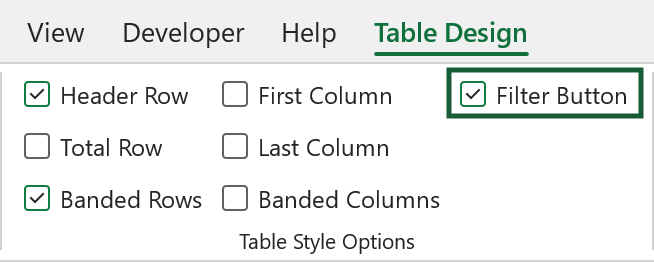
Table Names
A new table will automatically be assigned the name ‘Table’ followed by a sequential number, e.g. Table1, Table 2 and Table3.
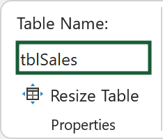
To change the name, edit the Table Name entry in the Table Design contextual tab.
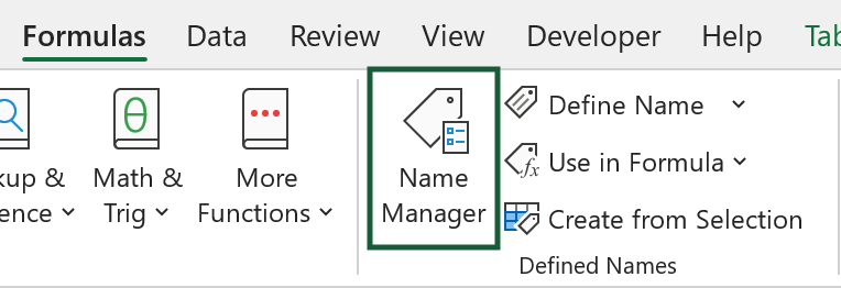
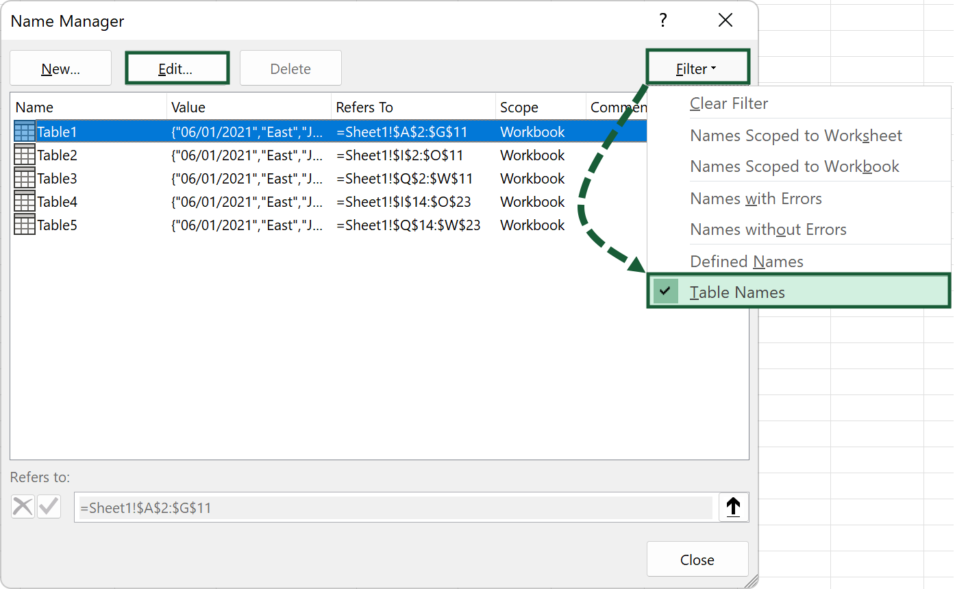
If you are batch renaming, instead of navigating to each table, select Formulas (tab) > Name Manager (button).
This window contains all your tables and named ranges. Click on Filter and then Table Names so only tables show. You can change a table name by highlighting one and clicking Edit.
Enter a new name and click OK.
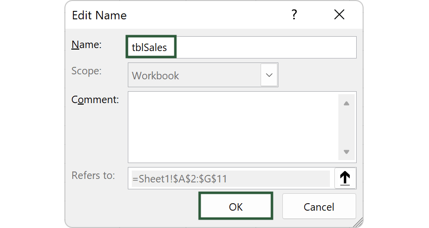
Table Name Rules
A table name must:
- start with a letter, underscore (_), or backslash ()
- be unique — it cannot clash with any other table name or named range
- be between (and including) one and 255 characters
- be formed of letters, numbers, underscores and full stops only
- not include spaces or other special characters
- not be a cell reference
- not be named C, c, R, or r
Excel does not distinguish between uppercase and lowercase letters, so Table1 and table1 are deemed the same, for example.
Header Name Rules
The rules are much looser for header names, as you can use any characters you want, but they can only be a maximum of 255 characters. If you attempt to go beyond this, the rest will be truncated without warning.
Select a Table in the Name Box
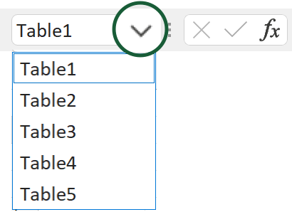
To the left of the formula bar is the name box. Click on the dropdown icon to unveil a list of all the workbook’s tables (and named ranges). Click one to activate it, no matter which worksheet it’s on.
Resize the Table
From the Ribbon
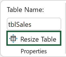
Activate a table and select Table Design (tab) > Resize Table (button).
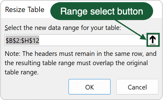
Edit the field manually with your updated cell range or choose a new range with your cursor. If you click on the range select button, it will bring up the same window you temporarily see when you select with the cursor alone.
With the Resize Handle
All tables have a small blue triangle in the bottom-right corner—this is the resize handle.
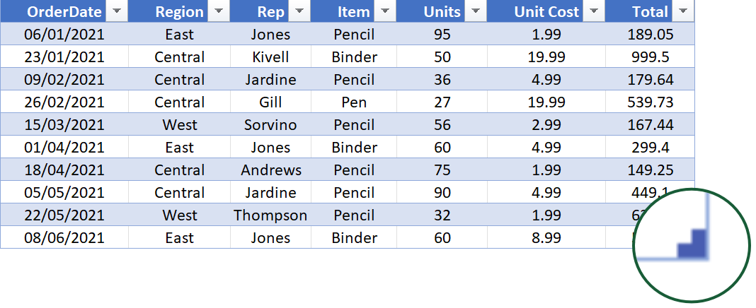
Hover over it for the cursor to change into a double-headed arrow. Left-click and hold whilst dragging downwards to expand the table or upwards to shrink it.

Any data sat below the table will be absorbed if you expand it. Whereas shrinking it will remove the data from the table.
Tables Expand Automatically
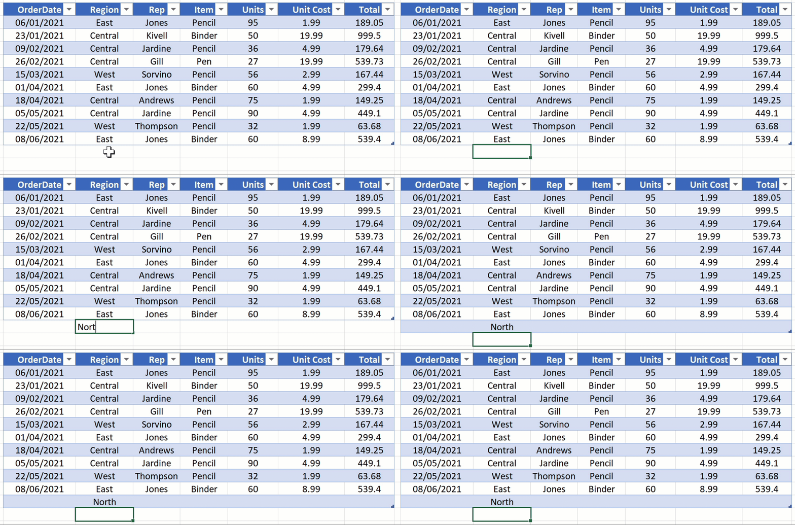
Any values you enter directly below or to the right of a table will trigger a new row or column.

Insert Rows or Columns
Instead of typing a new value to add a row or column, select one or more cells in the table and right-click to bring up the menu. Hover over Insert and several options will unveil. They will vary slightly depending on the position of the cell(s) you’ve chosen.
For the following, x and y represent the number of columns and rows in the cell selection, respectively:
Table Columns to the Left inserts x number of table columns to the left of the selection.
Table Columns to the Right inserts x number of table columns to the right of the selection.
Table Rows Above inserts y number of table rows above the selection.
Table Row Below inserts y number of table rows below the selection

Delete Rows or Columns
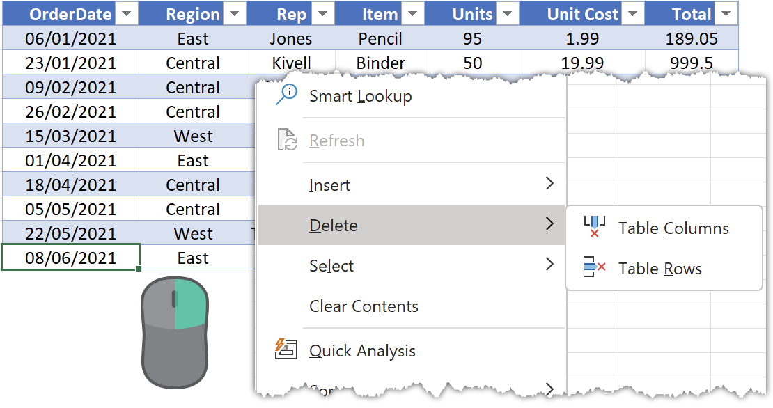
Similar to inserting, select a cell(s), right-click and hover over Delete to choose between Table Columns and Table Rows.
Select Table Parts
Select a Column
Hover over the top of a column header to turn the cursor into a down arrow. Left–click to select the entire data; click again to select the header and total as well.
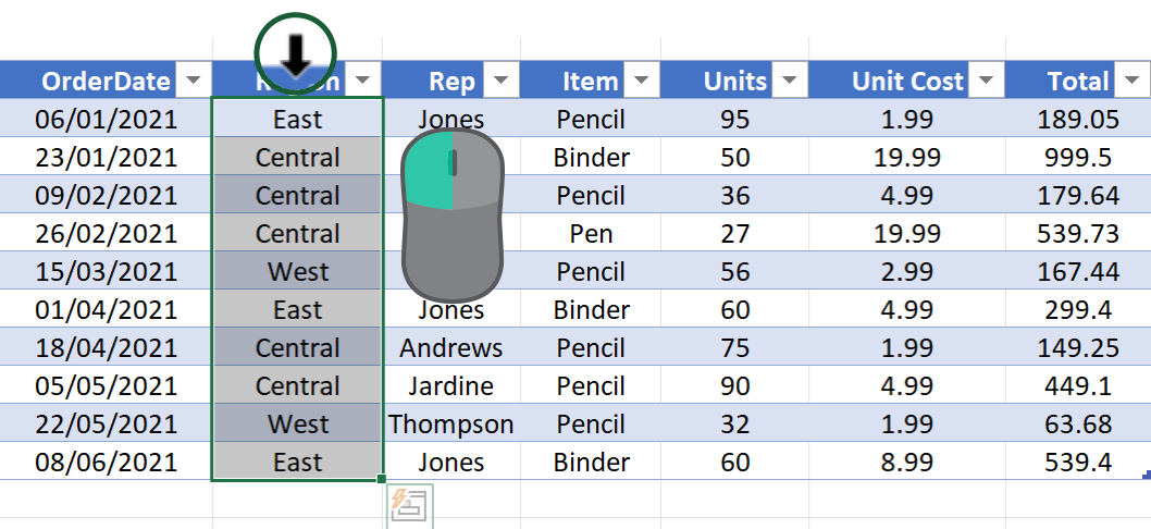
Alternatively, activate any cell in the column and press Ctrl + Space to select the data. Repeat this to include the header and total.
Select a Row
Hover over the leftmost of a row to turn the cursor into a right-pointing arrow. Left–click to select the entire row.
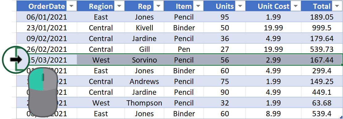
Alternatively, activate any cell in the row and press Shift + Space to select the data.
Select the Data
Hover over the top-left of a table to turn the cursor into a diagonal arrow. Left-click to select the data; click again to also include the header and total row.
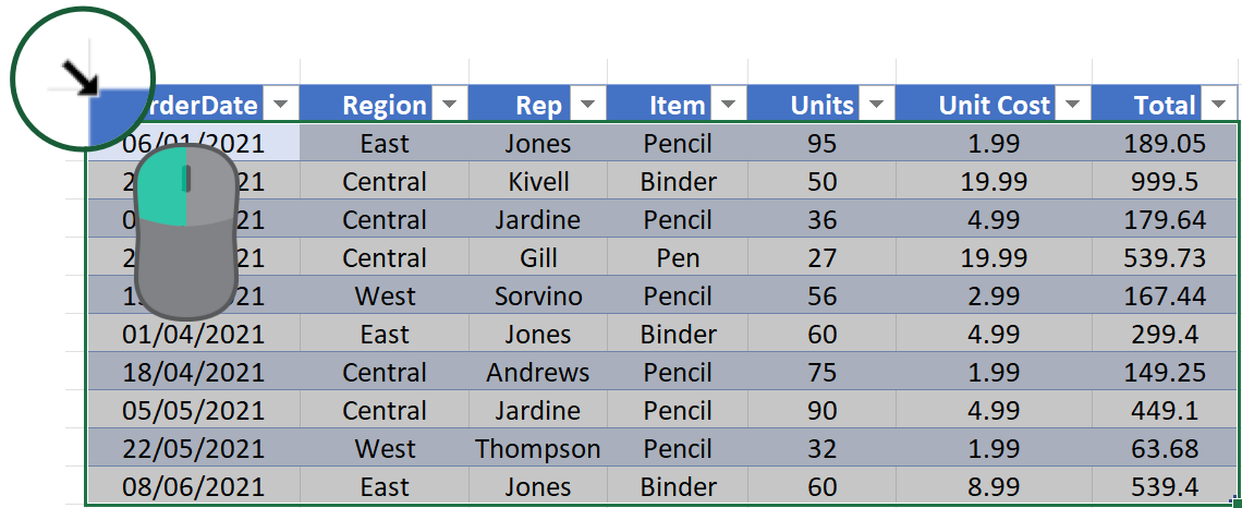
Alternatively, activate any table cell and press Ctrl + A (or Ctrl + Shift + Space) to select all the data. Do it again to include the header and total row.
Select the Header Row
Hover over the leftmost of the header row to convert the cursor into a right-pointing arrow. Then left–click to select it.

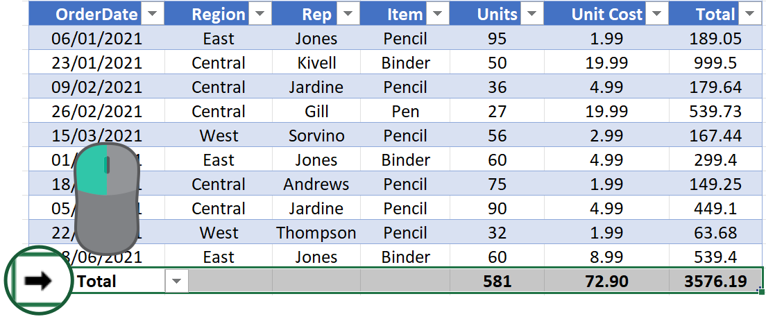
Select the Total Row
Hover over the leftmost of the total row to convert the cursor into a right-pointing arrow. Then left–click to select it.
Move a Table
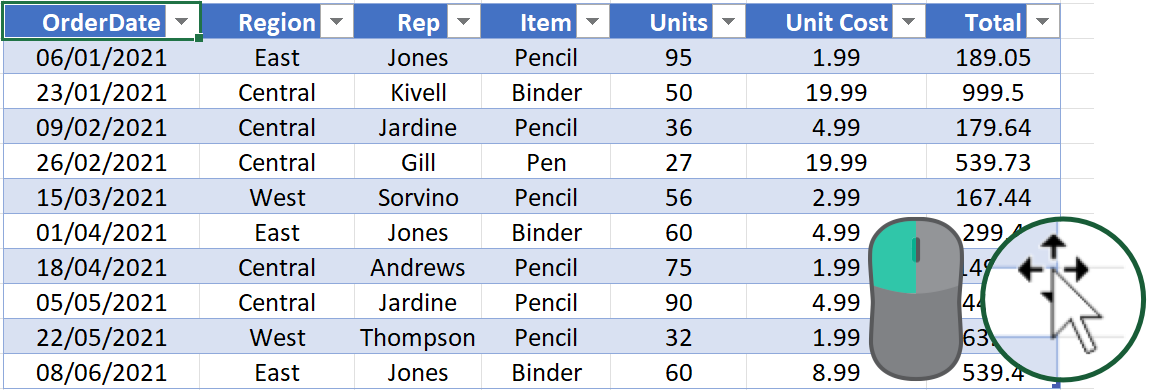
Activate a table and hover the cursor over one of the sides—it will change into a four-way directional arrow. Left–click, hold and drag to move the table to another location on the worksheet.
Summarize with PivotTable
Activate a table and select Table Design (tab) > Summarize with PivotTable (button) to insert a pivot table.
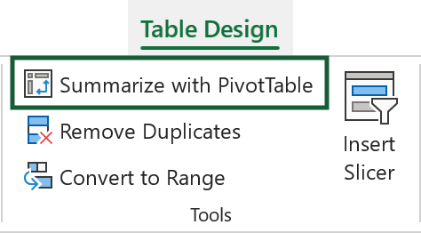
This button is the same as selecting Insert (tab) > PivotTable (button). It doesn’t offer anything additional.
To learn more about PivotTables, check out the guide at Exceljet.
Remove Duplicate Values
Activate a table and select Table Design (tab) > Remove Duplicates (button) to launch the Remove Duplicates window. Here, you can remove duplicate values from one or more columns.
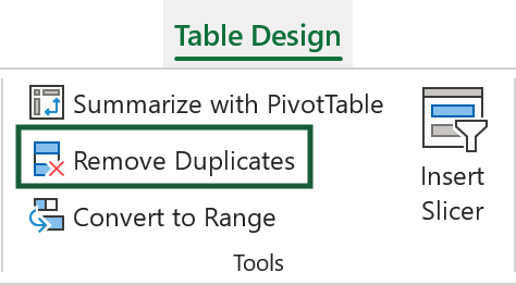
This button is the same as selecting Data (tab) > Remove Duplicates (button). It doesn’t offer anything additional.
To learn more about Remove Duplicates, check out the guide at Excel Easy.
Convert a Table to a Range
If you don’t want your data housed in a table along with the benefits it gives you, can convert it to a normal range.
Select Table Design (tab) > Convert to Range (button) to bring up a dialog box.

Click Yes to convert the table to a range.
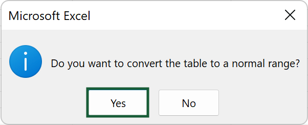
The range will lose the table features but retain its formatting.
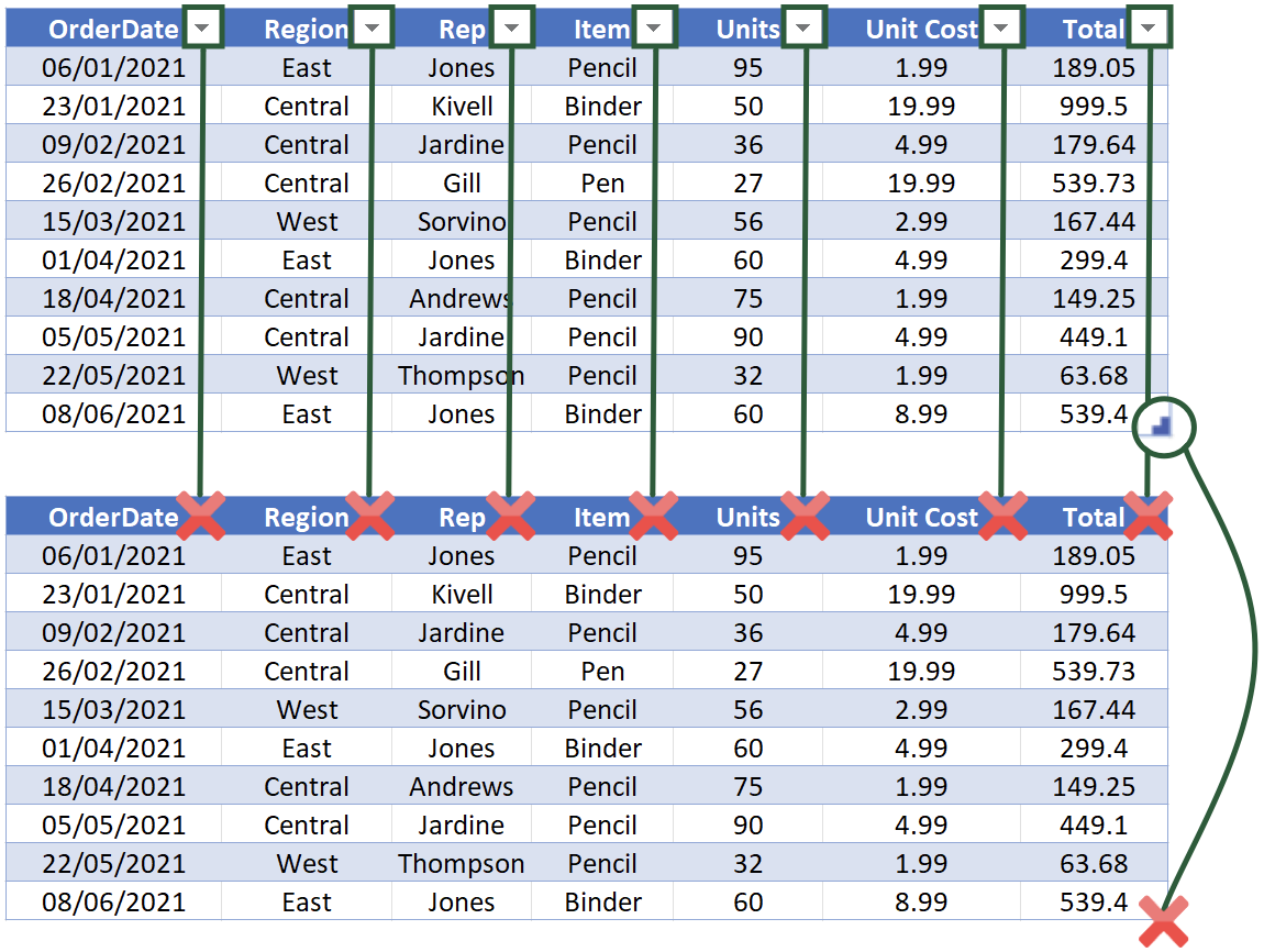
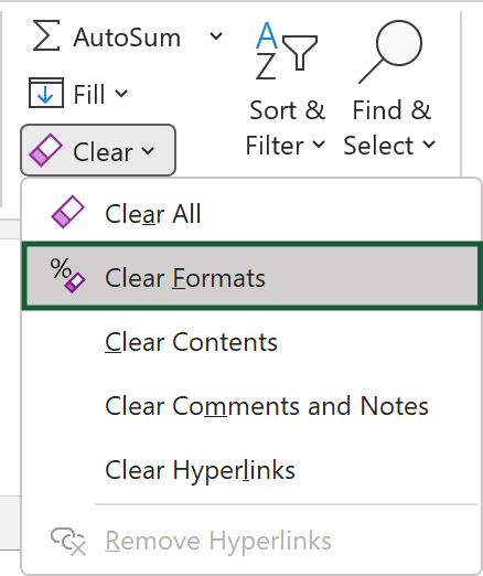
To remove this, select Home (tab) > Clear (dropdown)> Clear Formats (button).
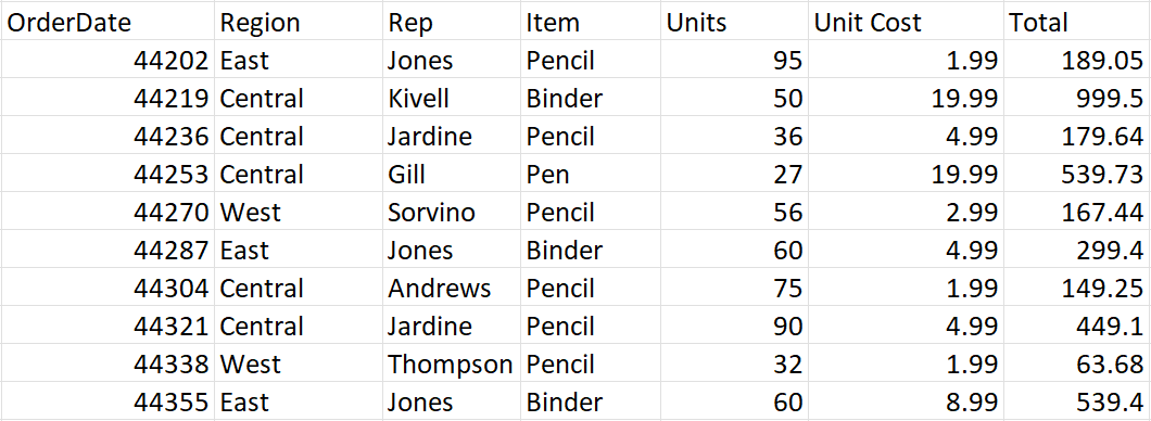
Your data will be stripped of all formatting.
In case you accidentally do this, press Ctrl + Z to undo the last action.
Insert a Slicer
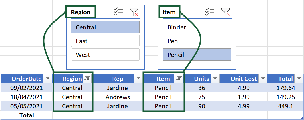
Slicers are interactive controls for filtering tables. They’re a friendlier alternative to column filter buttons, as they have a fixed presence on the worksheet.
On the Table Design tab, select Insert Slicer.
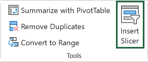
Tick the checkboxes for the columns you want a slicer for, and then click OK.
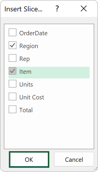
The slicers will appear on the worksheet, allowing you to filter the table accordingly.
Customise the Table Style
If you don’t want the default blue table theme, select Table Design (tab) to find the Table Styles gallery.
There’s a range of predefined styles to choose from. You can either use the spinner to quickly navigate by row or click More to unveil the whole set.

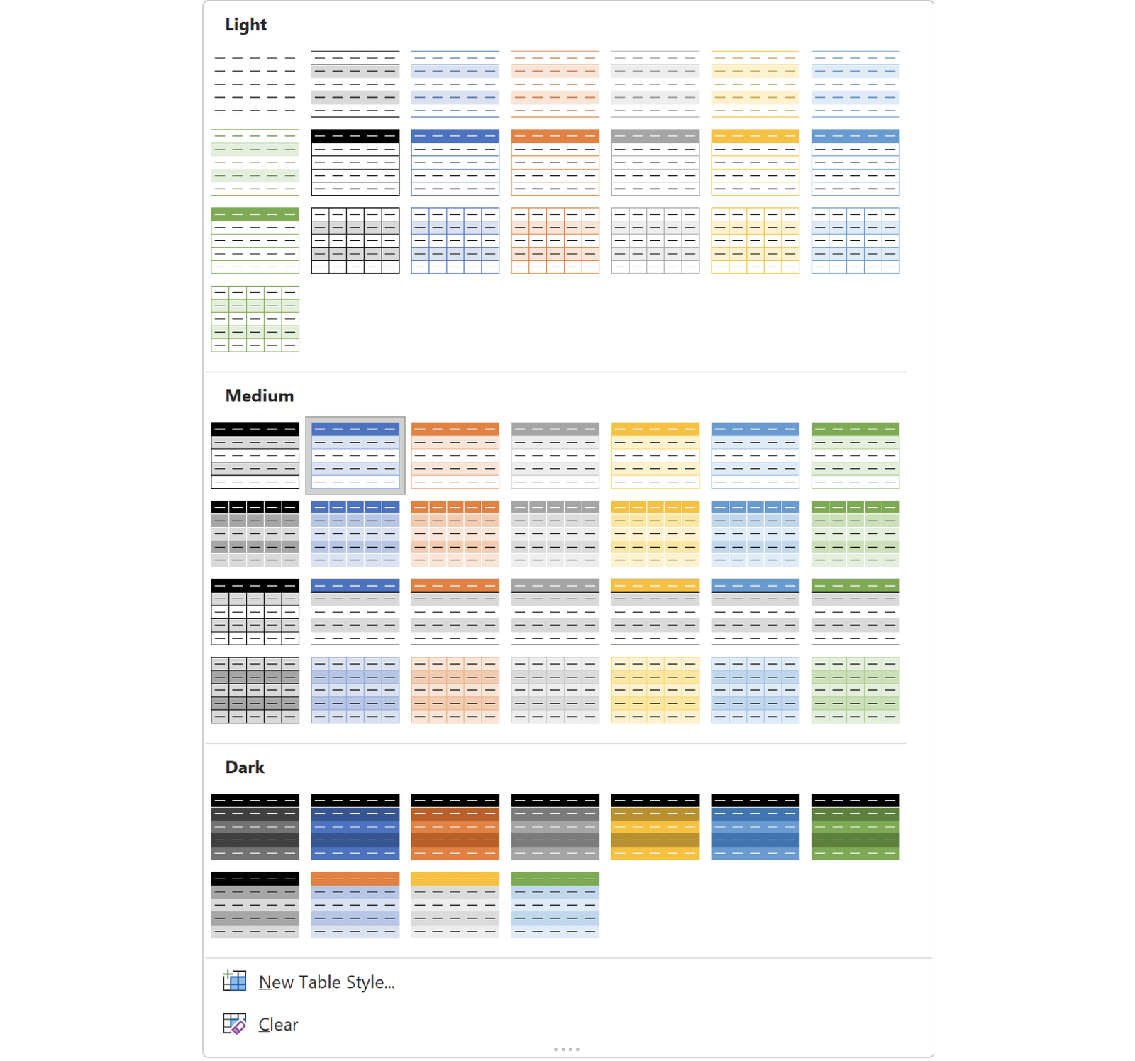
Another option is to select Home (tab) > Format as Table (dropdown). Don’t be fooled by the name—the gallery is almost identical and can be used to create new tables or apply styles to existing ones.
Custom Table Styles
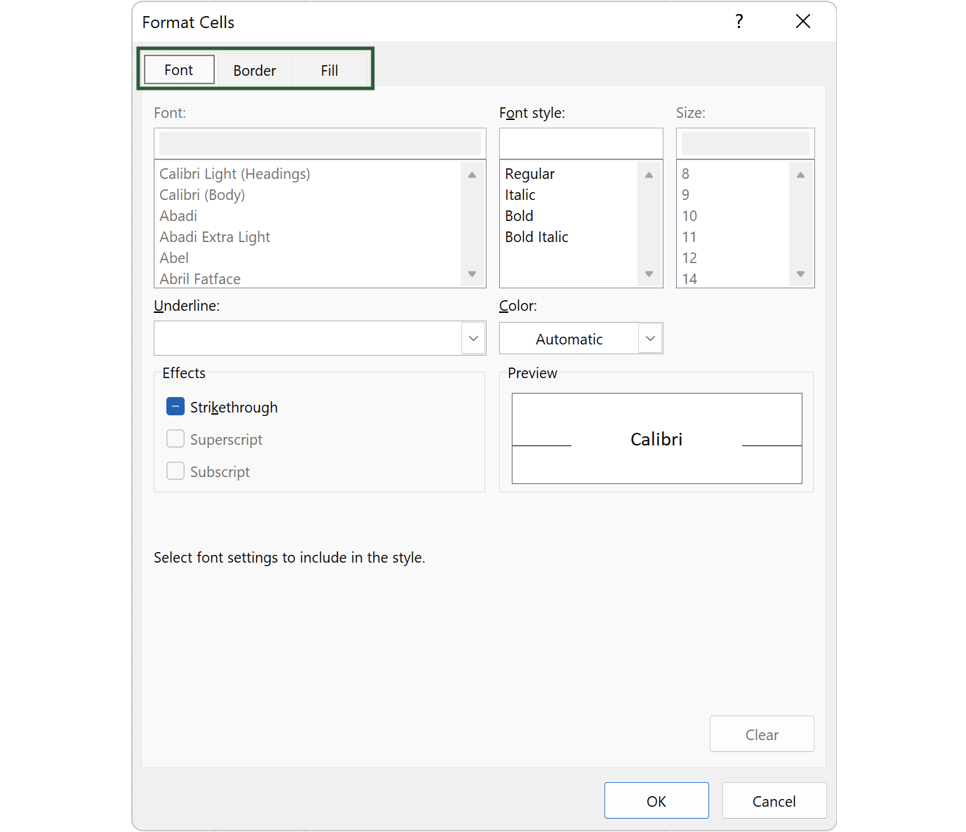
Click New Table Style to create your own theme. The window contains a list of table elements you can edit.
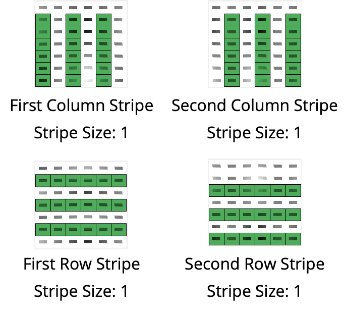
The elements with ‘Stripe’ in their names have a contextual dropdown that changes the number of consecutive stripes. The default is 1.
Highlight one and click Format.
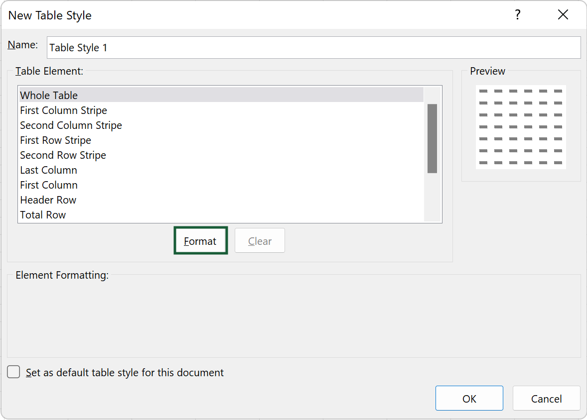
The Format Cells window opens, allowing you to set the font, border and fill colour.
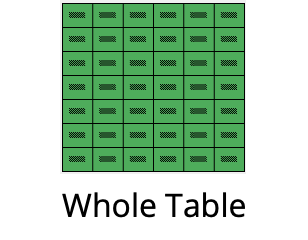
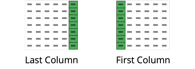
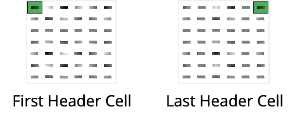
Each table element is previewed below and uses green fill and borders to show which part it affects.

Structured Referencing
The concept of cell referencing is probably entrenched in you. However, tables use something else called structured referencing.
With this, names identify table parts instead of cell ranges, making them more reader-friendly. Another advantage is when a table expands or shrinks, you don’t have to update any reference to reflect this.
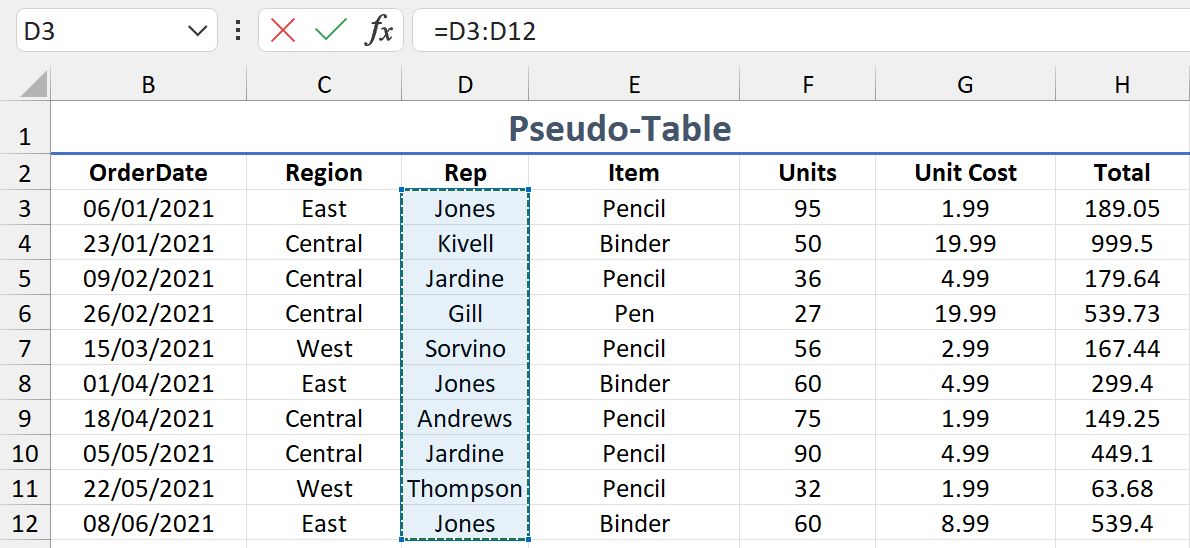
If you weren’t using a proper table, typically you’d reference a column with a formula like =D3:D12.
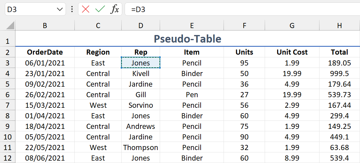
Or, before dynamic arrays were introduced, you would reference each cell individually. For example, =D3, =D4, and =D5.
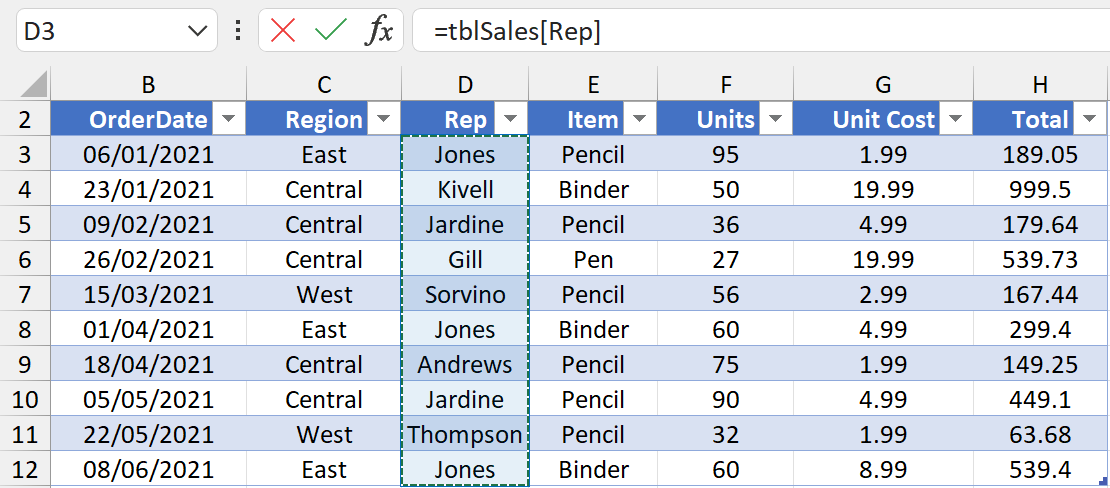
A table, however, allows you to use =tblSales[Rep].
Structured Reference Examples
The following examples show how to reference parts of a table with structured references.
Examples of Active Row Structured References
Reference the active row:
=table_name[@]
=tblSales[@]
Reference the active row of a column:
=table_name[@column_name]
=tblSales[@OrderDate]
Reference the active row of multiple columns:
=table_name[@[from_column_name]:[to_column_name]]
=tblSales[@[OrderDate]:[Region]]
Examples of Data Structured References
Reference the data (1 of 2):
=table_name
=tblSales
Reference the data (2 of 2):
=table_name[#Data]
=tblSales[#Data]
Reference the header row and data:
=table_name[[#Headers],[#Data]]
=tblSales[[#Headers],[#Data]]
Reference the data and total row:
=table_name[[#Data],[#Totals]]
=tblSales[[#Data],[#Totals]]
Reference the header row, data, and total row:
=table_name[#All]
=tblSales[#All]
Examples of Column Structured References
Reference the data of a column (1 of 2):
=table_name[column_name]
=tblSales[OrderDate]
Reference the data of a column (2 of 2):
=table_name[[#Data],[column_name]]
=tblSales[[#Data],[OrderDate]]
Reference the header row and data of a column:
=table_name[[#Headers],[#Data],[column_name]]
=tblSales[[#Headers],[#Data],[OrderDate]]
Reference the data and total row of a column:
=table_name[[#Data],[#Totals],[column_name]]
=tblSales[[#Data],[#Totals],[OrderDate]]
Reference the header row, data, and total row of a column:
=table_name[[#All],[column_name]]
=tblSales[[#All],[OrderDate]]
Reference the data of multiple columns:
=table_name[[from_column_name]:[to_column_name]]
=tblSales[[OrderDate]:[Region]]
Examples of Header Structured References
Reference the header row:
=table_name[#Headers]
=tblSales[#Headers]
Reference the header row of a column:
=table_name[[#Headers],[column_name]]
=tblSales[[#Headers],[OrderDate]]
Reference the header row of multiple columns:
=table_name[[#Headers],[from_column_name]:[to_column_name]]
=tblSales[[#Headers],[OrderDate]:[Region]]
Examples of Total Structured References
Reference the total row:
=table_name[#Totals]
=tblSales[#Totals]
Reference the total row of a column:
=table_name[[#Totals],[column_name]]
=tblSales[[#Totals],[OrderDate]]
Reference the total row of multiple columns:
=table_name[[#Totals],[from_column_name]:[to_column_name]]
=tblSales[[#Totals],[OrderDate]:[Region]]
Pseudo-Table and Table Tests
Let’s do a comparison of the three aforementioned methods.
Below shows a range of data that is contained in a pseudo-table.
The same data is also housed in a table.
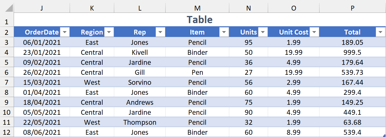
Several tests are carried out to observe the effect on the output of formulas that reference the Rep column.
The Cell Method references each cell individually, whereas the Range Method uses a single formula to spill the whole range.
Moreover, the Structured Reference Method is only applicable to the table, and this points to the column name.
Delete Rows 6 to 9
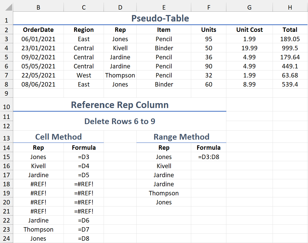
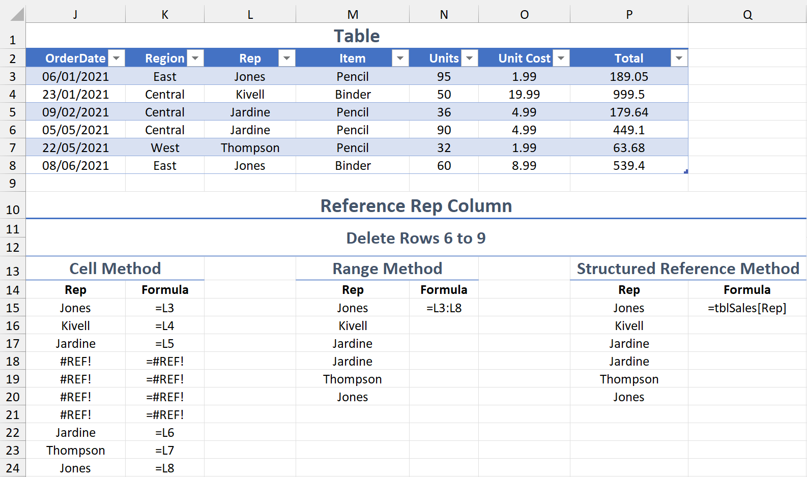
After deleting rows 6 to 9, the missing values are replaced by #REF! errors in both cell methods. This doesn’t occur in the range or structured reference methods though, as they adjust to the new ranges.
Insert 4 Rows Below Row 5
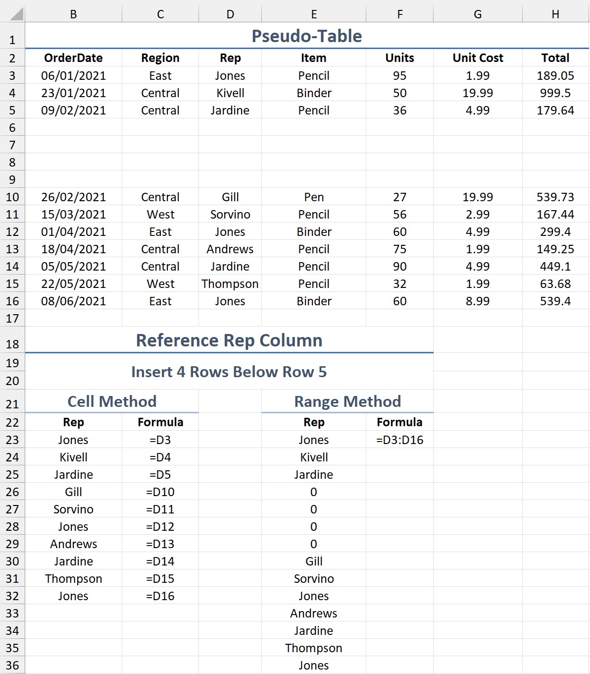

After inserting 4 rows below row 5, a gap appears. This is not reflected in the cell methods though, which update to skip these cells but reference the ones after.
The range and structured reference methods do recognise the gaps but replace the blank values with zeros.
Add a New Value to the Rep Column
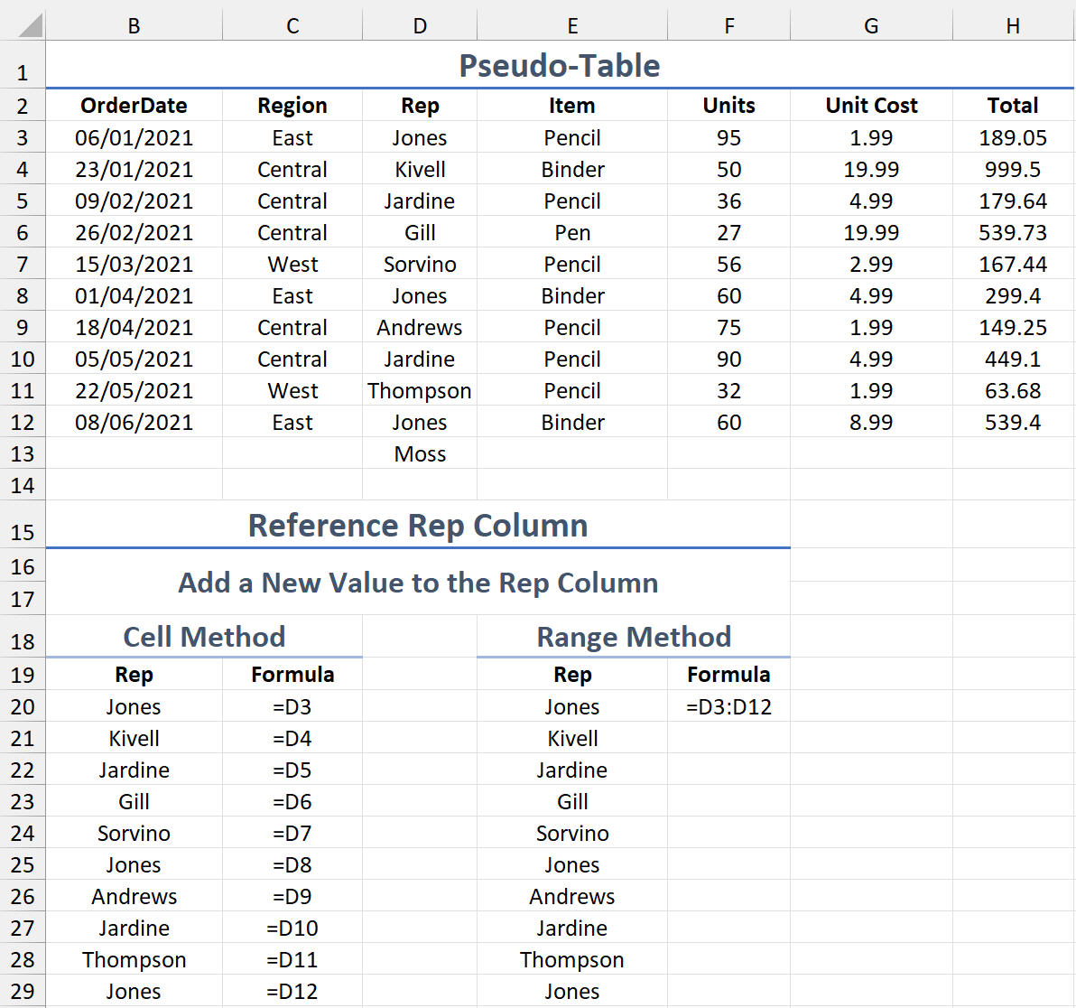
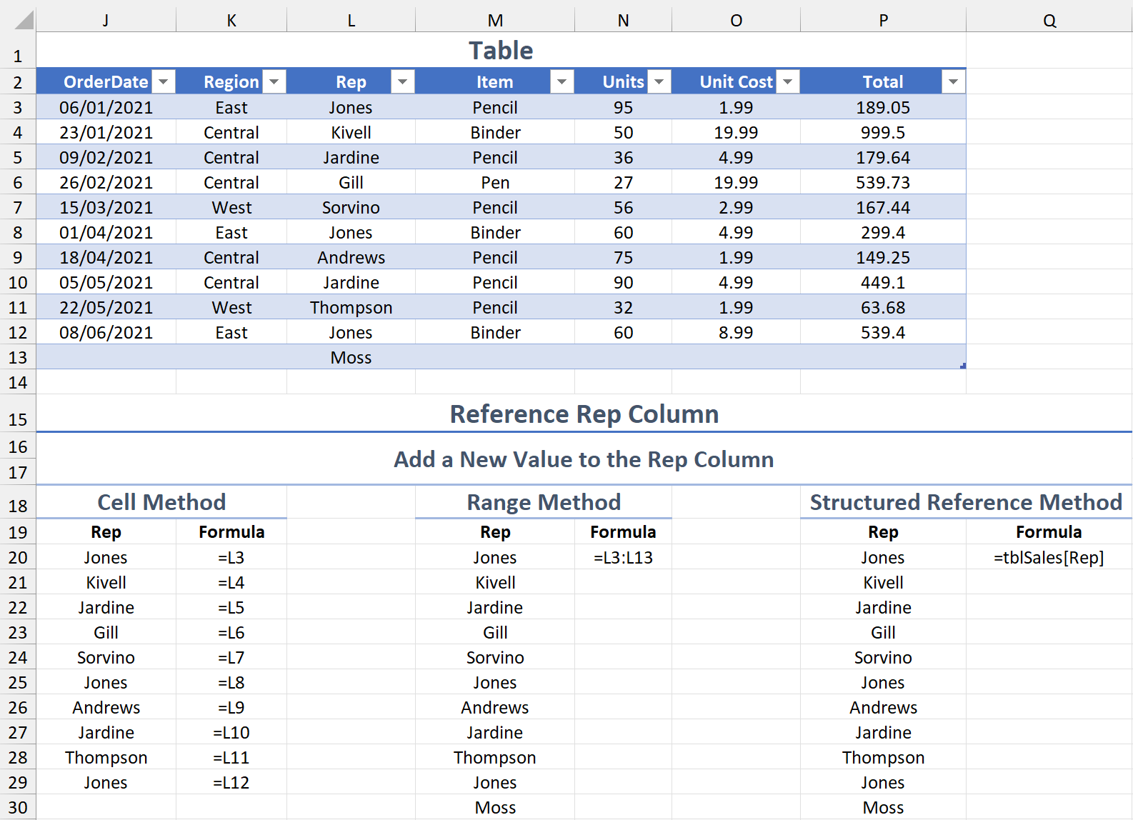
Moss is added to the Rep column but goes unnoticed by the cell methods, which require new formulas underneath the existing ones.
Although this is the case for the range method in the pseudo-table example, it isn’t in the other, as it automatically tweaks the reference. The structured reference method also returns the same result.
General Remarks
These tests prove that tables are more efficient and reliable than not using them. In truth, using a table and referencing with a range held up well, but named columns still trump ranges from a readability perspective.
Each action may have been separate, but just imagine the mess you’d cause to a referenced pseudo-table if you executed one after another!
Calculated Columns
There’s no need to type out, copy and paste, or drag the fill handle down to plant the same formula in every row of a column. This is automatically done for you after entering just one anywhere in a column. Another advantage is any new row you add will include the formula.

Turn Off Calculated Columns
If you don’t want calculated columns, you can turn them off.
Select File (tab)> Options (button)> Proofing (button) > AutoCorrect Options (button) to open the AutoCorrect window.

On the AutoFormat As You Type tab, untick the Include new rows and columns in table checkbox to enter values directly below or to the right of a table without them being absorbed.
Untick the Fill formulas in tables to create calculated columns checkbox to stop formulas from automatically populating a column.
Column Headers Stay Visible
An active table’s header names stay in sight even as you scroll down the worksheet. They replace the column letters temporarily until you scroll back up or click off the table.

Referencing Using AutoComplete
AutoComplete (also called IntelliSense) is a small pop-up box that makes referencing table parts a lot easier, as it reduces the need to type them manually.
Just putting equals followed by the first letter of the table name brings up a list of suggestions. You can go further for more accuracy.
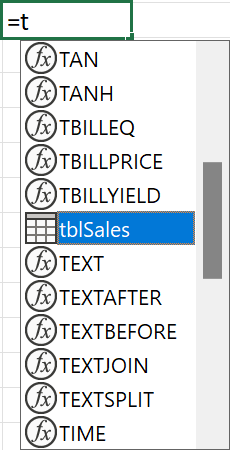
Highlight the chosen table and press the tab key. This autocompletes the name.
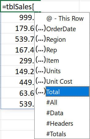
Add an opening square bracket to see all the table’s items. Again, select one and press tab — then finish with a closing square bracket.

Summary
Tables are great, aren’t they?
Here are a few of the advantages you’ve just learned about:
- Tables use structured references instead of cell ranges, making them more efficient and reader-friendly.
- Calculated columns prevent the need to type a formula more than once.
- Tables expand automatically when data is added directly below or to the right of them.
- Tables have sort and filter options built-in, as well as slicers.
- Column headers stay visible even when they’re outside the current view.
- Tables can be customised—there are over 50 pre-defined styles or you can create your own.
If you’re not already using tables, consider doing so. Despite being a fixture since Excel 2007 (and before under a different name), they remain one of the most underused features.
It’s time to change that.
