How to Use VLOOKUP in Excel

The VLOOKUP function enables you to search for a value in one column and return another from the same row in a different column. As it works from top to bottom, the ‘V’ stands for vertical.

Arguably, it’s the most famous function in Excel and one of the first you’ll learn. It has been ever-present since the program’s birth in 1985!

This article explains how to use it and the options it provides.

CONTENTS

· Download Workbook
· Syntax
· The Basics
  ∘ Standard VLOOKUP
  ∘ Only the First Match Is Returned
  ∘ Column Positions Matter
  ∘ Right to Left Lookup (1)
  ∘ Right to Left Lookup (2)
· Approximate Match
· Errors
· Wildcards
· Case Sensitivity
  ∘ Case-Insensitive Lookup
  ∘ Case-Sensitive Lookup
· Final Words

Download Workbook

This file contains all the examples explained in the article.

💾 VLOOKUP-Examples.xlsb

Syntax

=VLOOKUP(lookup_value, table_array, col_index_num, [range_lookup])

All arguments are required except [range_lookup].

lookup_value—the value to look for in the first column of the table_array.

table_array—the range containing the value to search for and the one to return.

col_index_num—the column number of the table_array containing the return value.

[range_lookup]—specify a logical value to return either an approximate or exact match:

TRUE/1 — returns an approximate match.
FALSE/0 — returns an exact match.

This is an optional argument so will default to TRUE if omitted.

The Basics

Standard VLOOKUP

We have a customer table and want to find the email address of Eric Rampy.

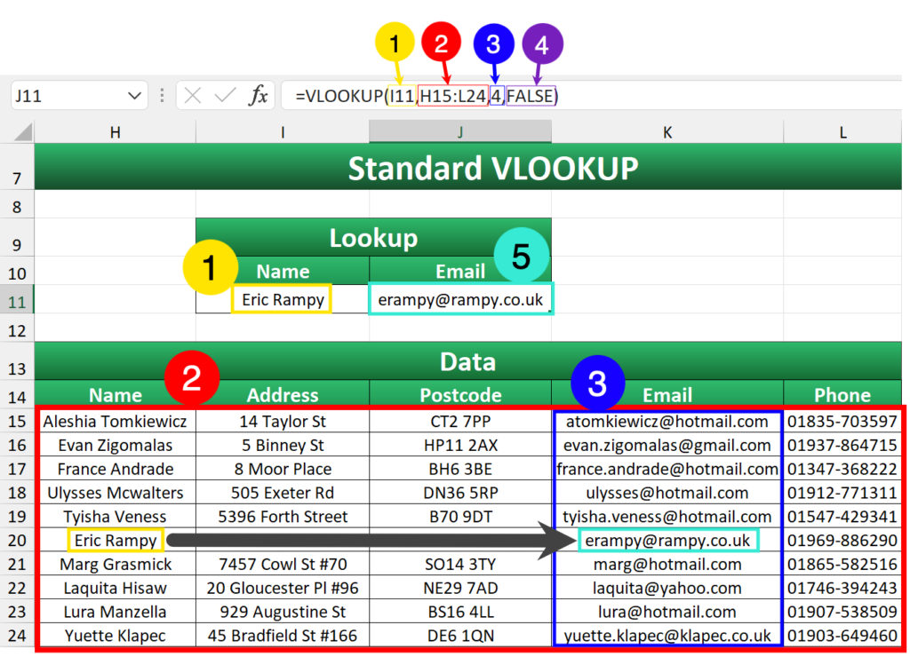
=VLOOKUP(I11,H15:L24,4,FALSE)

1. The lookup_value references I11, which contains Eric Rampy.
2. The table_array is the entire customer data in H15:L24.
3. The col_index_num is 4, which corresponds to the Email column.
4. The [range_lookup] is FALSE to ensure an exact match is found.
5. The formula in J11 returns erampy@rampy.co.uk.

Only the First Match Is Returned

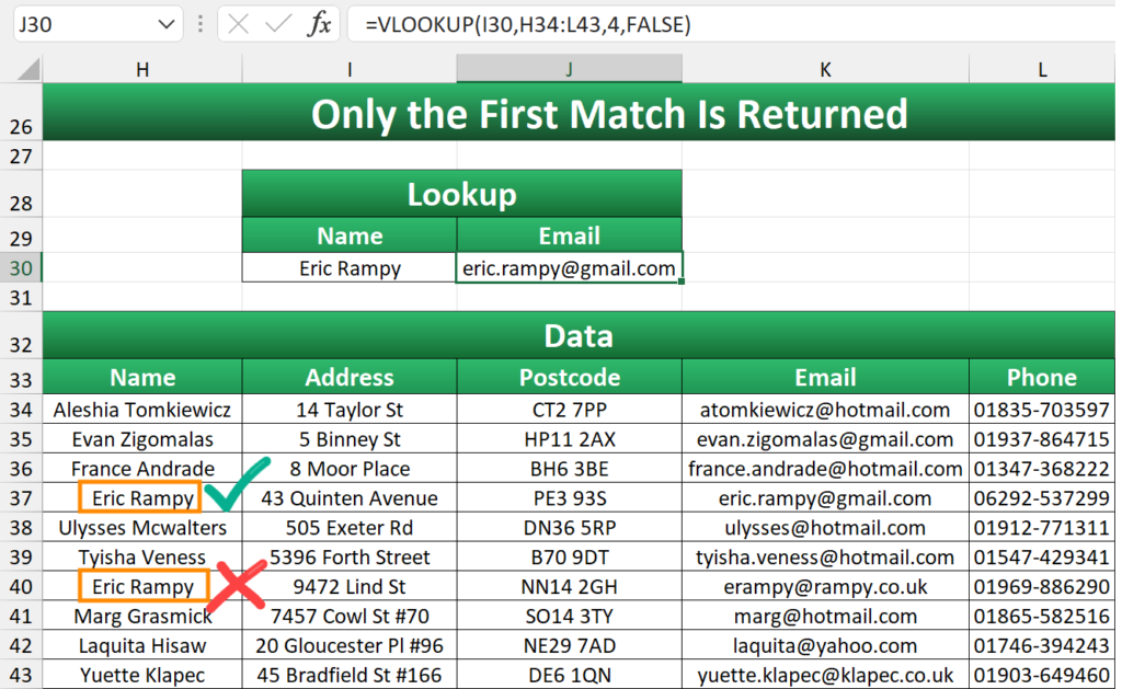
VLOOKUP only returns the first matching row, so any duplicates below it will be ignored.

In this example, the original email address for Eric Rampy is no longer returned as it is preceded by an identical value in the Name column.

Column Positions Matter

The lookup_value must be in the leftmost column of the table_array and the return value to the right of it.

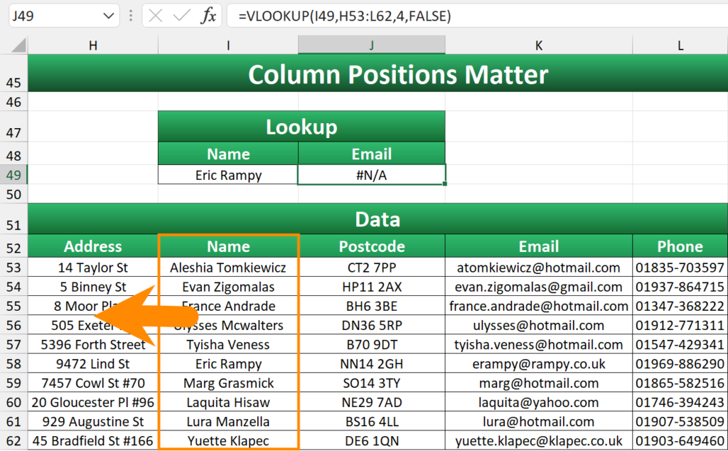
As the Address column is now first, Eric Rampy does not appear so a #N/A error occurs.

Right to Left Lookup (1)

Sometimes it’s not appropriate to change the column order of the existing data. To circumvent this, one option is to duplicate the return column and place it after the lookup one.

Here, we want to search for the email address and return the name.

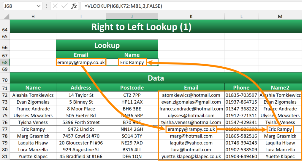
=VLOOKUP(I68,K72:M81,3,FALSE)

The lookup_array begins in the Email column and the final value is returned from Name2, which sits at the end referencing the values of Name.

Right to Left Lookup (2)

A better option is to combine VLOOKUP with CHOOSE.

=CHOOSE(index_num, value1, [value2], ...)

CHOOSE allows you to reference each column individually to generate an array. The value is then retrieved from the column set in VLOOKUP’s col_index_num.

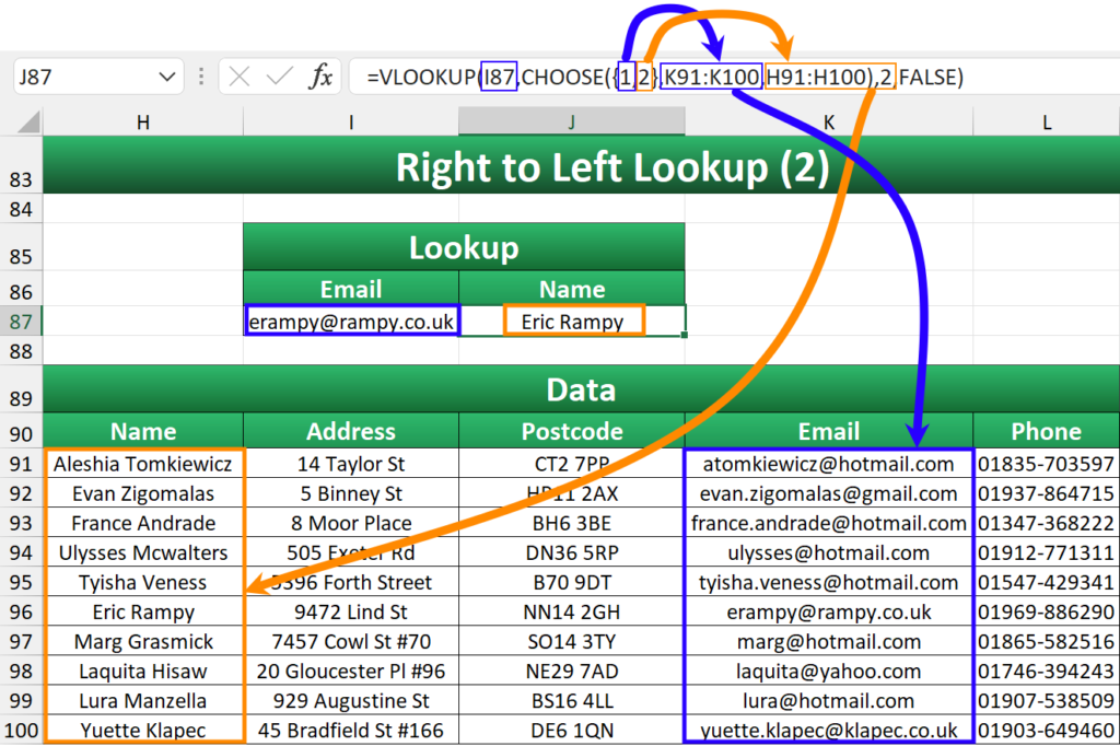
=VLOOKUP(I87,CHOOSE({1,2},K91:K100,H91:H100),2,FALSE)

The lookup column doesn’t necessarily have to be referenced first, but it does require an index_num of 1.

This method has another benefit as well: if you add a new column to the table, the formula won’t break.

The examples hereon use Excel Tables instead of cell references to reference data. If you’re not familiar with these, check out Exceljet’s guide.

Approximate Match

Setting [range_lookup] to TRUE returns an approximate match. Despite being the default, it’s unlikely you’ll want this the majority of the time. It’s useful for numeric data though, where typically there is more variation so you’re less interested in finding a specific figure.

In this example, the table contains grade boundaries that correspond to degree classifications.

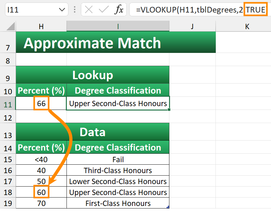
=VLOOKUP(H11,tblDegrees,2,TRUE)

We want to find the degree classification for 66%. An exact match would return a #N/A error as it doesn’t exist in the table. However, using an approximate match means it finds the nearest value that is less than the one being looked up. This is 60%, which is the minimum threshold for Upper Second-Class Honours.

Your data must be sorted in ascending order for an approximate match to work. Otherwise, you will get unusual results.

Errors

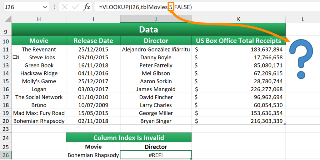
VLOOKUP will result in an error when something has gone wrong. Here are some examples:

#REF! — the col_index_num is greater than the number of columns in the table_array.

#N/A — the lookup_value is not found in the table_array.

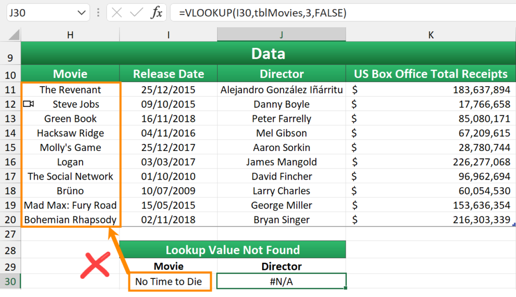
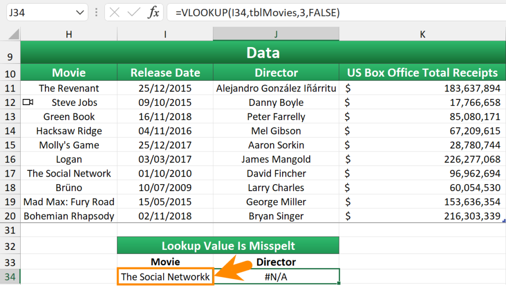
#N/A — the lookup_value is misspelt or has an extra space.

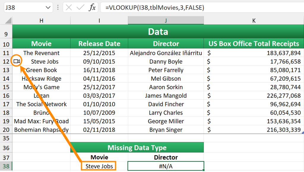
#N/A — the lookup_value is missing a data type.

#N/A — the lookup_value mismatches the table_array entry’s data type.

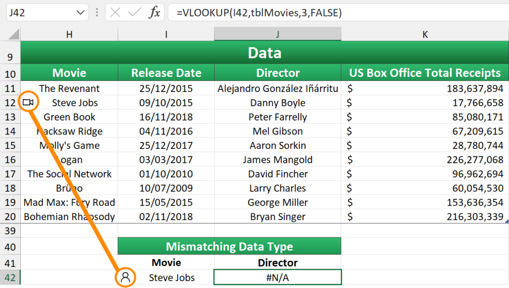
Steve Jobs is a person but there’s also a movie with the same name. These are not considered equal, even though the content is identical in each cell.

To trap these errors, wrap the IFERROR function around the VLOOKUP statement to replace them with something else.

The following will return Not Found:

=IFERROR(VLOOKUP(I38,tblMovies,3,FALSE),"Not Found")

This will return an empty string:

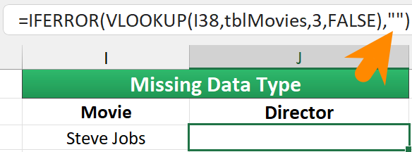
=IFERROR(VLOOKUP(I38,tblMovies,3,FALSE),"")

Wildcards

VLOOKUP supports wildcards, which are characters that take the place of text, so you can widen the scope of your lookup.

• An asterisk (*) represents any number of characters.
• A question mark (?) represents one character.
• A tilde (~) is the precursor for a literal character, in cases where * or ? are looked up.

These examples show how each wildcard can be used and the results they return. The original data is housed at the top, and each lookup table contains a few values to search for so the corresponding numbers are returned.

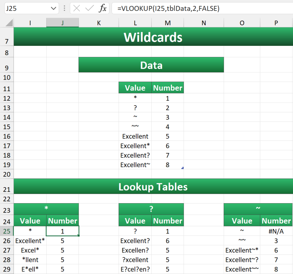
Examples:

• Ex*ent returns 5 (Excellent) as the asterisk fills in for ‘cell’.
• E?cel?en? returns 5 (Excellent) as the question marks fill in for ‘x’, ‘l’, and ‘t’, respectively.
• Excellent~~ returns 8 (Excellent~) as the second tilde is the literal character.

Case Sensitivity

By default, VLOOKUP performs a case-insensitive lookup, meaning it finds the first match in a range irrespective of whether it’s uppercase, lowercase or mixed case. To circumvent this, it can be used in conjunction with EXACT.

EXACT checks two text strings to see if they’re the same case. TRUE is returned if they are — FALSE if not.

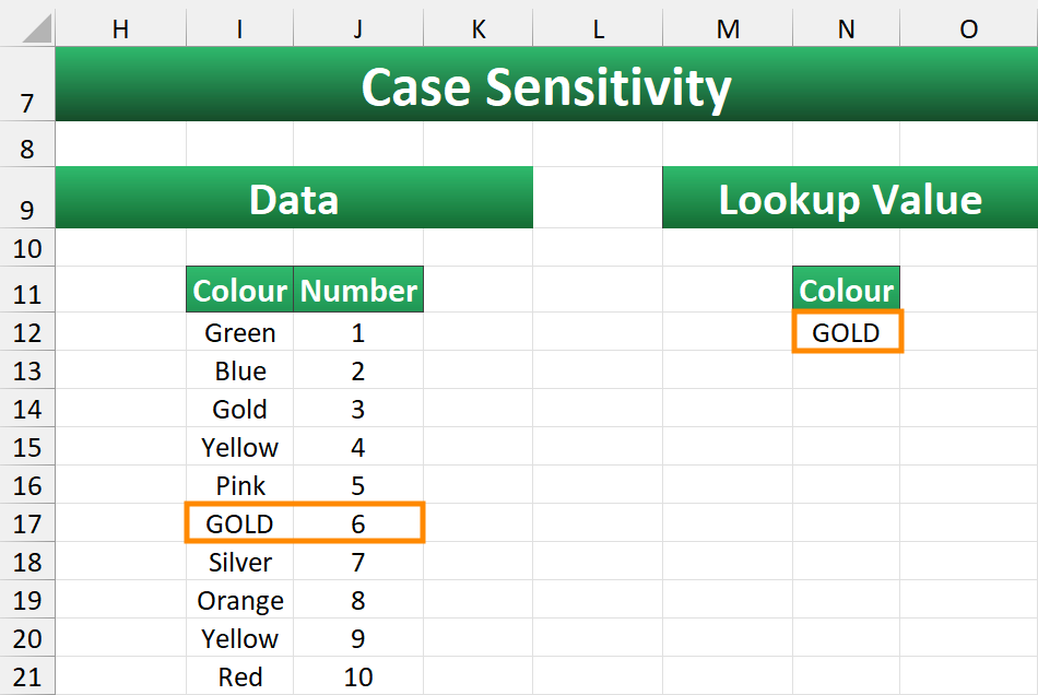
=EXACT(text1, text2)

A table called tblColours contains a set of colour names alongside corresponding numbers. We want to look up GOLD from N12 and return the adjacent number.

Case-Insensitive Lookup

A standard VLOOKUP formula retrieves the number of GOLD from tblColours. As Gold appears before GOLD, 3 is returned.

=VLOOKUP(N12,tblColours,2,FALSE)

Case-Sensitive Lookup

This time, the lookup_value is TRUE while the lookup_array uses CHOOSE to hold the EXACT statement and the Number column.

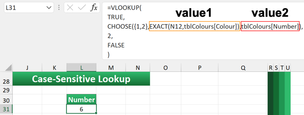
=VLOOKUP(
TRUE,
CHOOSE({1,2},EXACT(N12,tblColours[Colour]),tblColours[Number]),
2,
FALSE
)

In value1, EXACT(N12,tblColours[Colour]) evaluates to an array of 10 logical elements, with the sixth being the sole TRUE value. This is the position of GOLD in the Colour column.

Now we know the lookup element, we can return the corresponding value in value2, which is 6.

Final Words

Congratulations! You’ve just learnt a useful function that will help you a lot on your Excel journey. Practice, experiment, and explore the different ways of using it. However, don’t get too comfortable.

Mastering VLOOKUP is the gateway to bigger and better methods, namely INDEX/MATCH and XLOOKUP. These have advantages that cannot be overlooked.

I strongly recommend you move on to these once you’re ready for greater efficiency and flexibility.