How to Create an Excel Calendar

Calendars are useful for scheduling events, constructing to-do lists, and managing projects. Many applications exist for mobile and desktop, such as Outlook, iCloud Calendar, and Google Calendar. Whilst these are feature-packed and great for day-to-day use, nothing beats an Excel calendar for true customisation.
This article looks at three modern approaches to building a calendar in Excel.
𝗖𝗢𝗡𝗧𝗘𝗡𝗧𝗦

• Download Workbook
• Controls
  ∘ Start Day (Dropdown)
  ∘ Year (Spinner)
  ∘ Month (Dropdown)
  ∘ Highlight Weekends (Checkbox)
  ∘ Display Days Outside Year (Checkbox)
  ∘ Display Days Outside Month (Checkbox)
  ∘ Display Week Numbers (Checkbox)
• Week Numbers
• Week Headings
• Year/Month Headings
• Main Formulas
  ∘ Example 1
  ∘ Example 2
  ∘ Example 3
• Conditional Formatting
• Creating and Viewing Events
  ∘ Add a Recurring Event
  ∘ Add a Non-Recurring Event
  ∘ Dynamic Event Viewer
• Scenario Testing
• Final Words
Download Workbook

Use an Excel for Microsoft 365 desktop version for maximum compatibility.
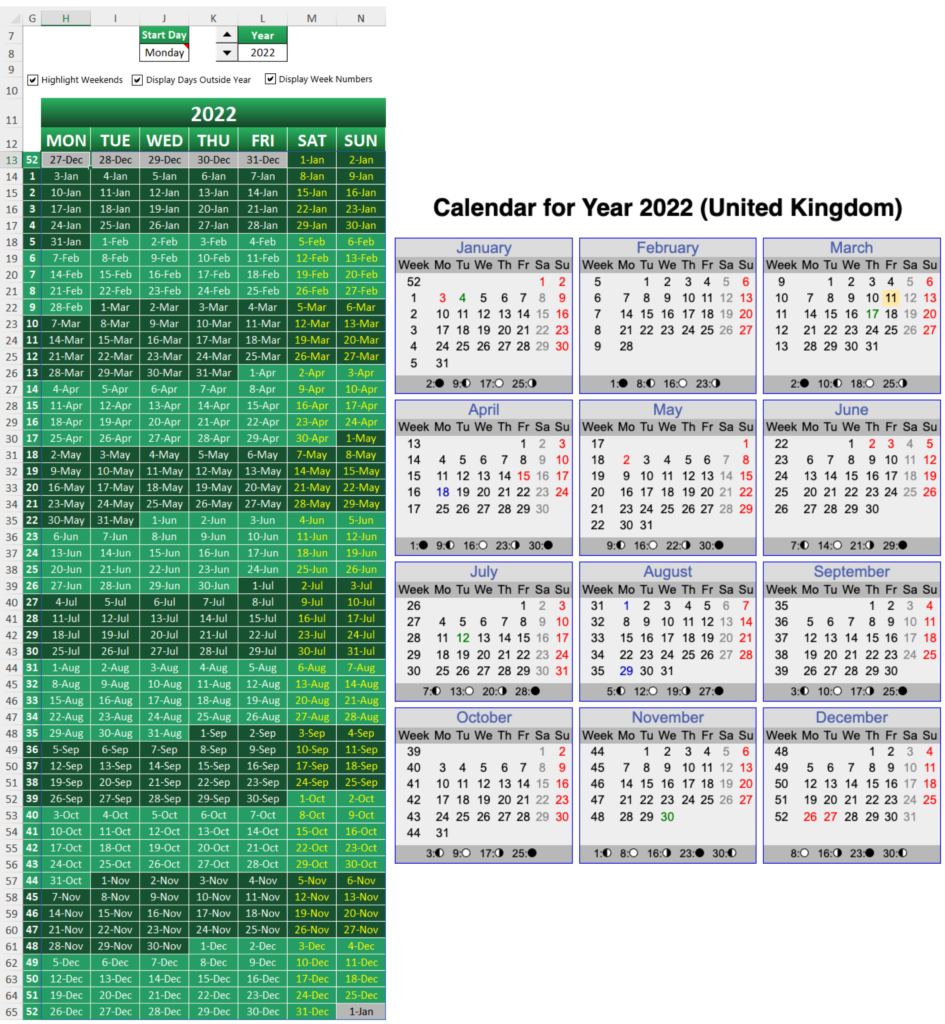
There are three worksheets, with each containing a different calendar type:
- Example 1 — an annual calendar that displays the year as a continuous set of months
- Example 2 — a monthly calendar that displays a single month only
- Example 3 — an annual calendar with separated months and the ability to create and view events
Before delving into the main formulas, let’s start by looking at the peripheral features they have in common.
Controls
Several controls exist to alter the calendar output. A named range represents the linked cell on the worksheet.
Start Day (Dropdown)

The day each week starts from—either Monday or Sunday.
e1_.dd1.StartDay—J8 in Example 1e2_.dd1.StartDay—I8 in Example 2e3_.dd1.StartDay—H8 in Example 3
Year (Spinner)

The year the calendar represents.
e1_.sp1.Year—L8 in Example 1e2_.sp1.Year—M8 in Example 2e3_.sp1.Year—K8 in Example 3
The spinner allows a range between 1901 and 9998. Data validation also ensures no year outside this boundary can be entered.
Why?
Excel doesn’t recognise dates before 1st January 1900 or after 31st December 9998. It also has a known issue where 1900 is incorrectly treated as a leap year.
Setting 1901 as the starting point ensures there’s no issue with any loose days that precede the start of the new year.
Month (Dropdown)

The month the calendar represents.
e2_.dd2.Month—K8 in Example 2
Highlight Weekends (Checkbox)

If ticked, days that fall on Saturday or Sunday are highlighted yellow.
e1_.ck1.HighlightWeekends—J9 in Example 1e2_.ck1.HighlightWeekends—I9 in Example 2e3_.ck1.HighlightWeekends—M9 in Example 3
Display Days Outside Year (Checkbox)

If ticked, days that fall outside the year are shown.
e1_.ck2.DisplayDaysOutsideYear—K9 in Example 1
Display Days Outside Month (Checkbox)

If ticked, days that fall outside the month are shown.
e2_.ck2.DisplayDaysOutsideMonth—K9 in Example 2e3_.ck2.DisplayDaysOutsideMonth—O9 in Example 3
Display Week Numbers (Checkbox)

If ticked, the week numbers appear in the far-left column, adjacent to the days.
e1_.ck3.DisplayWeekNumbers—L9 in Example 1e2_.ck3.DisplayWeekNumbers—M9 in Example 2e3_.ck3.DisplayWeekNumbers—Q9 in Example 3
Each checkbox has a linked cell containing
TRUEorFALSE, but the custom cell format;;;ensures these values are invisible.
Week Numbers
Let’s dissect the Example 1 week numbers formula, which is almost identical across the three calendars.

It starts by checking the value of e1_.ck3.DisplayWeekNumbers is TRUE. If so, the [value_if_true] argument is triggered.
SWITCH() holds the Start Day value in the expression argument. This means if the dropdown is set to Monday, result1 is returned.

Inside WEEKNUM(), INDEX() extracts the week numbers of the dates in the farthest left column. The [return_type] is 21, which corresponds to Monday.
The prefixing double hyphen converts the result to an array of values. This is necessary because WEEKNUM() doesn’t spill ranges by default like other functions.
WEEKNUM ( serial_number , return_type )
INDEX ( array, row_num, column_num )
When Sunday is set as the start day, result2 is returned. This part is trickier than the last because of the way Excel handles System 1 week numbers.
If =WEEKNUM(--INDEX(H13#,,1),17) was used, it would not return the correct weeks, as F13 starts with 53 and jumps to 2 below.

Where is week 1?
Let’s digress for a moment and understand how the different week systems work.
In the vast majority of the Americas, the week officially begins on Sunday. Across Europe though, it’s Monday, which follows the ISO 8601 international standard.

The rule for week 1 in the American system is simple: it starts in the first week containing 1st January.
ISO 8601 rules stipulate the following for week 1:
• it is the first week with at least four days belonging to January
• it contains 4th January and the first Thursday of the year
• the first day is the Monday closest to 1st January
If the return_type argument is omitted, WEEKNUM() assumes Sunday (System 1) is the first day of the week.

Notice how Monday appears three times and Sunday twice? Excel 2007 and earlier versions only contained options 1 - Sunday and 2 — Monday. That changed in Excel 2010 with the addition of eight others.
All but one are based on System 1, with the anomaly being 21 - Monday, which uses System 2 to adhere to the aforementioned ISO 8601 standard. ISOWEEKNUM() also returns the same result.
I posted about week numbers on LinkedIn recently and gave an example.

Two calendars are present — one based on a start day of Sunday (System 1), and the other on Monday (System 2). Both use formulas that reference the dates in column K, however, the first week number is wrong in the former. That’s because the reference doesn’t cover Q17, which contains 01/01/2022.
At the bottom is a grid showing all week number possibilities for the first 16 days. The column pairs that output identical results are shaded separate colours.
You can now understand why week 53 was being returned. This means another method is required, consisting of an IF() statement that checks if 1st January is featured in each row.

Behind this is MMULT(), which returns the matrix product of two arrays.
In array1, (H13#=DATE(e1_.sp1.Year,1,1)) checks for 1st January of the chosen year and generates a set of TRUE and FALSE values.
The + (OR) operator joins (H13#=DATE(e1_.sp1.Year+1,1,1)), which does the same for the following year.
Because of the presence of the second condition, TRUE and FALSE are coerced into 1 and 0 values. It results in an array that determines where 1st January is situated on the calendar.
{0,0,0,0,0,0,1;0,0,0,0,0,0,0;0,0,0,0,0,0,0;0,0,0,0,0,0,0;0,0,0,0,0,0,0;0,0,0,0,0,0,0;0,0,0,0,0,0,0;0,0,0,0,0,0,0;0,0,0,0,0,0,0;0,0,0,0,0,0,0;0,0,0,0,0,0,0;0,0,0,0,0,0,0;0,0,0,0,0,0,0;0,0,0,0,0,0,0;0,0,0,0,0,0,0;0,0,0,0,0,0,0;0,0,0,0,0,0,0;0,0,0,0,0,0,0;0,0,0,0,0,0,0;0,0,0,0,0,0,0;0,0,0,0,0,0,0;0,0,0,0,0,0,0;0,0,0,0,0,0,0;0,0,0,0,0,0,0;0,0,0,0,0,0,0;0,0,0,0,0,0,0;0,0,0,0,0,0,0;0,0,0,0,0,0,0;0,0,0,0,0,0,0;0,0,0,0,0,0,0;0,0,0,0,0,0,0;0,0,0,0,0,0,0;0,0,0,0,0,0,0;0,0,0,0,0,0,0;0,0,0,0,0,0,0;0,0,0,0,0,0,0;0,0,0,0,0,0,0;0,0,0,0,0,0,0;0,0,0,0,0,0,0;0,0,0,0,0,0,0;0,0,0,0,0,0,0;0,0,0,0,0,0,0;0,0,0,0,0,0,0;0,0,0,0,0,0,0;0,0,0,0,0,0,0;0,0,0,0,0,0,0;0,0,0,0,0,0,0;0,0,0,0,0,0,0;0,0,0,0,0,0,0;0,0,0,0,0,0,0;0,0,0,0,0,0,0;0,0,0,0,0,0,0;0,0,0,0,0,0,0}In array2, TRANSPOSE(COLUMN(H13#)^0) transposes the calendar column numbers and squares them by zero. As anything squared by zero equals one, {1;1;1;1;1;1;1} is produced. These are then multiplied by array1 to return 1 or 0 in a smaller array where each element represents a row. The IF() logical_test checks for 1 and results in the same number if TRUE.
{1;0;0;0;0;0;0;0;0;0;0;0;0;0;0;0;0;0;0;0;0;0;0;0;0;0;0;0;0;0;0;0;0;0;0;0;0;0;0;0;0;0;0;0;0;0;0;0;0;0;0;0;0}The regular Sunday (System 2) week numbers are returned in [value_if_false]. These fill in the 0 elements in the previous array, while 1 gets ignored.
{53;2;3;4;5;6;7;8;9;10;11;12;13;14;15;16;17;18;19;20;21;22;23;24;25;26;27;28;29;30;31;32;33;34;35;36;37;38;39;40;41;42;43;44;45;46;47;48;49;50;51;52;53}Week 1 will always represent the first row, but the last one will vary. For example, 2022 is a 53-week year, whereas 2023 is only 52.


Week Headings
The week headings are found at the top of each calendar and are all based on the same formula.

SWITCH() uses the Start Day value to decide which permutation to return. They are each stored as array constants so will spill across.
Year/Month Headings
In Example 1 and Example 3, the year headings reference the respective spinner cells e1_.sp1.Year and e2_.sp1.Year.

Example 2 uses TEXTJOIN() to concatenate the month and year separated by a space.

In Example 3, DATEVALUE() converts the string comprising the month and year to a recognised date, which the cell outputs as a month.

Main Formulas
Example 1
In H13, LET() holds several named values the calendar requires to function.

They are:
StartDate — the first date of the chosen year.
FirstDay — a number from 1 to 7 to identify when StartDate begins — based on a week beginning on Monday.
DayToNumber — converts the chosen Start Day to a number — Monday to 1 and Sunday to 7.
Calendar — generates the calendar according to the chosen year.
To accommodate all possibilities in Calendar, SEQUENCE() constructs an array of 54 rows and seven columns. StartDate is the starting value, but added to this is an IF() statement that calculates how many days precede 1st January.
If FirstDay is greater than or equal to DayToNumber, the calculation DayToNumber-FirstDay takes place. If not, then it’s DayToNumber-7-FirstDay.
Let’s say we have the calendar set to Sunday and 2022 as the Start Day and Year, respectively. The calculation would look like this:
FirstDay = 6
DayToNumber = 7

IF(
6>=7, logical_test
7-6, [value_if_true]
7-7-6 [value_if_false]
)
As 6>=7 is FALSE, it jumps to [value_if_false] where the result is -6. This means six days are subtracted from StartDate, so the whole calculation becomes 44562 − 6 = 44556. 44556 in regular date format is 26/12/2021, which is the first day of the calendar.

Now the names have been assigned values, the main calculation can take place.

Another IF() statement determines whether the calendar should be composed of 54 or 53 weeks. MAX(Calendar)-6 finds the largest date in the calendar and subtracts six days to land on the first day of the last week. YEAR() then extracts the year of this date and checks if it’s equal to the spinner value.
If TRUE, the 54-week Calendar is returned, otherwise, this name is chucked into an INDEX() statement to return 53.
It’s worth noting that not many years require 54 rows, as they occur in leap years when 1st January falls on the last day of the first week. Examples include 2000 and 2028 for a Sunday start week and 2012 and 2040 for Monday.

Example 2
This example uses largely the same formula as the last. However, it only outputs a single month, so a few adaptions are required.

A new name called MonthToNumber exists, and the month that matches the dropdown is converted to a number from 1to 12. It’s used in StartDate and Calendar to ensure the month value in DATE() can change.

Instead of 54 and 53 rows, this calendar deals with four, five and six. Another name called Calendar2 is required to handle the rare instance of February fitting into four rows exactly.

In the main calculation, the first part is altered from the previous example, as it subtracts six days from the maximum date of Calendar, and then extracts the month to see if it’s equal to MonthToNumber.
If so, Calendar outputs six rows. If not, another IF statement involving Calendar2 checks if cell K8 is equal to February and the first day of the fifth week doesn’t belong to it. In that case, only four rows are displayed, otherwise, it’s five.

Example 3
Example 2 set the foundation for this calendar type, as essentially it is 12 of those in the same worksheet with a few minor differences.

MonthToNumber doesn’t require SWITCH() to hold each month as each block only has one, so MONTH() extracts it from the heading.
Again, consideration had to be made for February, as it’s the only month that can fit perfectly into four rows. That’s why its formula is a little different.
Conditional Formatting
Without any colour, Example 1 would be dull and difficult to look at. As a visual enhancement, alternating colours help distinguish the separate months.
How is this done though?

Let’s say the calendar is set to 2022 with a Start Day of Monday. We’ll focus on the bottom two rules first.
MOD returns the remainder after a value is divided by a divisor. In this case, 12 is returned in the number argument as the date’s month in H13 is December. The calculation becomes 12 ÷ 2 = 6. 6 is not equal to 1 or 0, so nothing happens.

Two other rules that serve the same purpose but highlight the text yellow if the Highlight Weekends checkbox is ticked are also ignored.

This is where the two grey-based rules come in. The top one checks if Display Days Outside Year is switched on and displays black text on a grey background if it has. Conversely, the bottom displays the grey without any text if it’s switched off.

1st January starts in M13, so now the MOD() calculation is 1 ÷ 12 = 0.08. Anything above 0 counts as 1, so the dark green rule becomes true.
Jump to 1st February in I18 and the light green rule takes precedent, as the remainder of 2 ÷ 2 is 0.

Separate rules are necessary for the week numbers, but the same principles apply. Some rows contain the end of one month and the start of another, but the colour of each week cell will always match the adjacent one.

The top rule is responsible for ensuring nothing appears in the week number column if they are turned off, as well as stopping unnecessary formatting in the 54th row.

Example 2 has fewer rules, but there is one noticeable inclusion that makes use of TODAY() to highlight the current day in yellow.

Example 3 gets a bit messy, as separate rules are needed for each month, due to the use of absolute cell references.

The dark orange rule fills in the cells that have events belonging to the month. Whereas the washed-out one does the same for events outside the month.
They are also used in the dynamic event area and All Events table.

More details about the event system are explained in the next section.
Creating and Viewing Events
To take things to the next level, Example 3 allows you to create date-based events that are highlighted on the calendar.

They are stored in a table called e3_EventTable. Events can stretch to anything — meetings, deadlines, due payments, or special occasions (the examples were taken from Tree2mydoor).
The three columns are:
- DD/MM — the day and month of the event
- Date — the date of the event
- Event — the title of the event
You can add recurring and non-recurring events. The former will display for every year, whilst the latter will only show for a specific date.
Add a Recurring Event
- Type the day/month into the DD/MM column.
- Add a name for it in the Event column.
- Try changing the year with the spinner, and the event should repeat itself.
Add a Non-Recurring Event
- Override the Date column formula with your chosen date. This will prevent it from changing.
- Add a name for it in the Event column.
- Try changing the year with the spinner, and the event should not repeat itself.
Dynamic Event Viewer
To the left of the table is an area that outputs the details of any events that fall on the date of the active cell. This is done with the FILTER() function, which AI13 uses to return only the valid rows in the Event column.

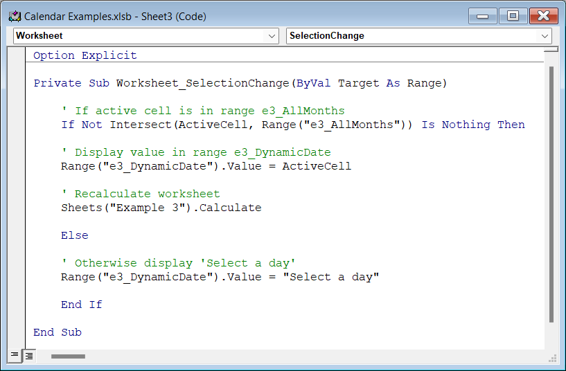
The named range e3_DynamicDate represents AI12, and it’s required by the VBA code to make the system operational.
Press Alt + F9 to open the VBA window and go into Sheet3 to view the procedure.

The Worksheet_SelectionChange event triggers whenever the active cell changes. It includes an If…Then…Else statement that:
- Checks if the active cell is in the range
e3_AllMonths. - If true, displays the date in
e3_DynamicDateand recalculates the worksheet. - If false, displays ‘Select a day’ in
e3_DynamicDate.
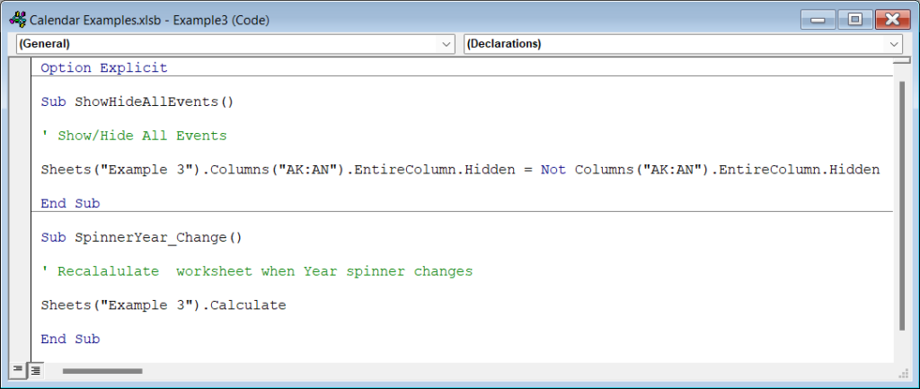
The Example3 module contains two other procedures.

ShowHideAllEvents is assigned to the Show/Hide All Events button, which toggles between the two states to make the events table visible or not.
SpinnerYear_Change recalculates the worksheet to ensure everything displays correctly.
Scenario Testing
It was important to do extensive testing on the calendar. After all, there are week numbers, start days and leap years to think about. No two years are the same.
Time and Date provided a useful online calendar for cross-checking purposes.

Final Words
I’m sure studying the calendar examples have enhanced your Excel knowledge and serve as handy templates for adapting to your needs.
Before building them, I found numerous examples strewn across the web, but almost all of them used old Excel methods. That meant a clunky formula for each day!
I’d like to think I’ve played a role in modernising the approach. It’s up to you now to take the calendars to the next level.
How will you be using them?
