How to Calculate Multiple Values in the Same Cell

The standard way of storing data in Excel is to have one cell for one value. However, a value might be composed of multiple parts — making it harder to work with. You might also copy content from a webpage, only to find it all packs into the same cell when you paste it.
For any scenario like this, you could use Text to Columns to separate each part according to a delimiter. Alternatively, Power Query has a Split Column By Delimiter feature that does the same thing.
But what happens if you don’t want to split the data?
As a rule of thumb, I wouldn’t recommend storing multiple values in a single cell. A key data principle is that values should be atomised. However, Excel is not a database, and the carte blanche nature of it means it’s commonly used in obscure ways.
This article looks at how you can perform calculations on single-cell data. This includes summing, counting and averaging numbers — as well as conditional and lookup statements.
Before We Start

Download the workbook containing the examples:
💾 Calculate-Values-in-Same-Cell-Examples.xlsb
You’ll need to be running a Windows Microsoft 365 copy of Excel. If not, you will run into problems with some or most of the examples — depending on your version.
One bit of advice for you that will help throughout:
To best understand the inner workings of a formula, click on a function argument in the tooltip and press F9 to convert it into a value. Ctrl + Z undoes this.

Examples Explained
There are three worksheet tabs: Part A, Part B and Part C.
Part A

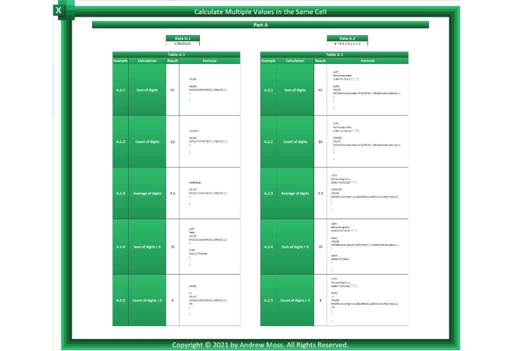
Data A.1 contains a value comprising 10 randomly ordered digits between zero and nine.

Table A.1 features five calculations performed on it.
Let’s look at the formula for example A.1.1:
=SUM(

VALUE(
MID(J10,SEQUENCE(1,LEN(J10)),1)
)

)
The MID function works by taking the value of cell J10 and converting it into a string for the text argument.
MID(text, start_num, num_chars)
MID(4789201635, {1,2,3,4,5,6,7,8,9,10}, 1)
start_num determines which character to begin from. Whilst this could be a fixed number, there are 10 to fetch. To avoid a lengthy formula, a shorter and cleverer method is required.
That’s why SEQUENCE is ideal for scenarios requiring an iterative looping process like this. It’s used to generate an array that equates to one row and 10 columns. If the character length changes, LEN(J10) ensures the correct figure is returned.
1 is stated for num_chars, as only a single-digit needs to be extracted for each iteration.
Collectively, the result of this is an array that is fed into the VALUE function to convert the indexes into numeric figures.
VALUE(text)
VALUE({"4","7","8","9","2","0","1","6","3","5"})
This is necessary for the SUM function to add each one to produce a final total of 45.
Calculation
=SUM(

{4,7,8,9,2,0,1,6,3,5}

)

Result
45
Examples A.1.2 and A.1.3 are almost identical, except the outer functions are COUNT and AVERAGE, respectively.
It’s worth noting that for counting characters, you’d probably be better off using the formula =LEN(J10). The mechanism that the LEN function uses differs in that it simply returns the number of characters. It doesn’t cycle through each one iteratively like the example does, which is a precursor for constructing something more complex.
A.1.4 and A.1.5 are conditional statements that only consider digits greater than five.
Let’s focus on A.1.4 first:
=LET(
Data,
VALUE(
MID(J10,SEQUENCE(1,LEN(J10)),1)
),

SUM(
(Data>5)*(Data)
)

)
LET allows you to store values under assigned names — most commonly known as variables. It’s good practice to do this if you have repetitive chunks of formula code.
It’s been used to store the same snippet you saw in the first example under the name Data.
In the next part, the calculation_or_name2 argument performs the calculation (Data>5)*(Data).
Each number is checked to see if it’s above five — resulting in an array of TRUE and FALSE indexes. These automatically coerce into 1 and 0 values when they’re multiplied by the original numbers.
The figures times by one return themselves, whereas the others produce zero.
SUM(
{0,1,1,1,0,0,0,1,0,0}
*
{4,7,8,9,2,0,1,6,3,5}
)
The SUM function then adds up the contents of the final array.
Calculation
SUM({0,7,8,9,0,0,0,6,0,0})

Result
30
Example A.1.5 counts numbers that are more than five. The formula is much the same as A.1.1, but the use of >5 turns it into a conditional statement.
=SUM(

--(
VALUE(
MID(J10,SEQUENCE(1,LEN(J10)),1)
)>5
)

)
You can’t add up an array of TRUE and FALSE values, so they must be converted to 1 and 0 values. To do this, an extra pair of brackets is wrapped around the VALUE statement with a preceding double-hyphen (--).
Perhaps you’re wondering: why did example A.1.4 not require this? The reason was: it involved two calculations sandwiched between an asterisk, so the -- was unnecessary.
Another thing that might confuse you is the use of SUM for a counting task. If COUNT was used instead, it would include zero values in the summation, making the final result 10.
Calculation
=SUM({0,1,1,1,0,0,0,1,0,0})

Result
4
Table A.2
You’ve just seen examples based on a value with consecutive digits. But what happens if it has an interrupted format?
Data A.2 contains the same numbers, except each is separated by a hyphen.

The solutions are based on removing the hyphens so the string only contains the relevant characters. This is done using SUBSTITUTE(Q10,"-",""), which has been stored as RemoveHyphens.
All instances where cell Q10 would usually be referenced in the formula have been replaced with this name.
Example A.2.1:
=LET(
RemoveHyphens,
SUBSTITUTE(Q10,"-",""),

SUM(
VALUE(
MID(RemoveHyphens,SEQUENCE(1,LEN(RemoveHyphens)),1)
)
)

)
Part B

This section is a step up from Part A, as it focuses on more flexible solutions.
If you have a bunch of values in a cell that vary in length, Part A will not suffice, as it’s for single characters only that follow a consistent pattern.
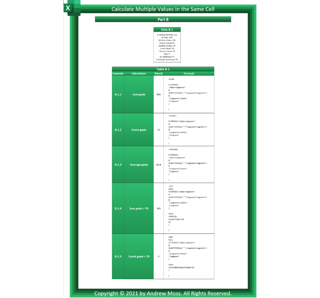
Value B.1 displays a list of the 10 all-time highest scorers in international football.

One thing the Table B.1 examples have in common is their use of the FILTERXML function.
It offers a convenient way of splitting values up based on a specific delimiter. Unlike Text to Columns though, which distributes the output across columns, FILTERXML allows you to create an XML code container for segmented data to be housed in. Each value is sandwiched between a pair of customised name tags. These can then be referenced in XPath expressions to limit the content returned.
Starting with example B.1.1:
=SUM(

FILTERXML(
"<data><segment>"
&
SUBSTITUTE(J10," ","</segment><segment>")
&
"</segment></data>",
"//segment"

)

)
The aim is to sum together all goals scored, but given the varying character lengths, how are the numbers extracted?
A skeleton structure is defined in the xml argument as a group of concatenated strings — each separated by an ampersand symbol (&).
An opening and closing tag are collectively known as an element. There are two required for this: one for the container and the other to represent a value.
To analogise, think of it this way: data is the house and segment is a room.
The first string consists of the opening tags <data><segment> followed by the second, which uses SUBSTITUTE to replace all spaces with </segment><segment>. When there are none left, the string ends with </segment></data>.
Put together and applied to Data B.1, the structure becomes:
<data>

<segment>Cristiano</segment>
<segment>Ronaldo</segment>
<segment>111</segment>
<segment>Ali</segment>
<segment>Daei</segment>
<segment>109</segment>
<segment>Mokhtar</segment>
<segment>Dahari</segment>
<segment>89</segment>
<segment>Ferenc</segment>
<segment>Puskás</segment>
<segment>84</segment>
<segment>Godfrey</segment>
<segment>Chitalu</segment>
<segment>79</segment>
<segment>Lionel</segment>
<segment>Messi</segment>
<segment>79</segment>
<segment>Hussein</segment>
<segment>Saeed</segment>
<segment>78</segment>
<segment>Pelé</segment>
<segment>77</segment>
<segment>Ali</segment>
<segment>Mabkhout</segment>
<segment>77</segment>
<segment>Kunishige</segment>
<segment>Kamamoto</segment>
<segment>75</segment>

</data>
Specifying the xpath as //segment extracts all values from segment elements.
An array is produced, and with SUM wrapped around the FILTERXML statement, each number is added up. The text entries are meaningless so have no bearing on the result.
Calculation
=SUM(

{“Cristiano”;”Ronaldo”;111;”Ali”;”Daei”;109;”Mokhtar”;”Dahari”;89;”Ferenc”;”Puskás”;84;”Godfrey”;”Chitalu”;79;”Lionel”;”Messi”;79;”Hussein”;”Saeed”;78;”Pelé”;77;”Ali”;”Mabkhout”;77;”Kunishige”;”Kamamoto”;75}

)

Result
858
Example B.1.4 makes use of a conditional statement to sum together all goal counts greater than 79.
The same FILTERXML code you just saw is stored under the name Data. This is then used in calculation_or_name2 to multiply each number by the condition.
SUM(

IFERROR(
(Data)*(Data>79),
0)

)
This converts to:
SUM(

IFERROR(
{"Cristiano";"Ronaldo";111;"Ali";"Daei";109;"Mokhtar";"Dahari";89;"Ferenc";"Puskás";84;"Godfrey";"Chitalu";79;"Lionel";"Messi";79;"Hussein";"Saeed";78;"Pelé";77;"Ali";"Mabkhout";77;"Kunishige";"Kamamoto";75}
*{TRUE;TRUE;TRUE;TRUE;TRUE;TRUE;TRUE;TRUE;TRUE;TRUE;TRUE;TRUE;TRUE;TRUE;FALSE;TRUE;TRUE;FALSE;TRUE;TRUE;FALSE;TRUE;FALSE;TRUE;TRUE;FALSE;TRUE;TRUE;FALSE},
0)

)
IFERROR replaces all the #VALUE! errors in the array with zeros to ensure the summation is successful.
SUM(
{#VALUE!;#VALUE!;111;#VALUE!;#VALUE!;109;#VALUE!;#VALUE!;89;#VALUE!;#VALUE!;84;#VALUE!;#VALUE!;0;#VALUE!;#VALUE!;0;#VALUE!;#VALUE!;0;#VALUE!;0;#VALUE!;#VALUE!;0;#VALUE!;#VALUE!;0},
)
The numbers are summed to yield a final result of 393.
Calculation
SUM(
{0;0;111;0;0;109;0;0;89;0;0;84;0;0;0;0;0;0;0;0;0;0;0;0;0;0;0;0;0}
)

Result
393
Example B.1.5 counts the goals that are above 79. It’s slightly different because it uses ISNUMBER to output TRUE or FALSE depending on whether the array index is a number. As a result, it doesn’t require IFERROR as there are no text strings involved.
SUM(
(ISNUMBER(Data))*(Data>79)
)
The calculation and result are:
Calculation
SUM({0;0;1;0;0;1;0;0;1;0;0;1;0;0;0;0;0;0;0;0;0;0;0;0;0;0;0;0;0})

Result
4
Part C

The final section looks at how lookup statements can convert nebulous data into something more understandable.
This example is based on a fictional property company that owns houses in several cities across the UK and rents them out to individuals.
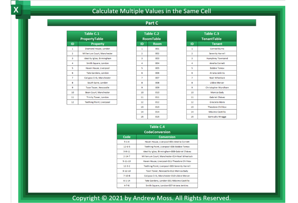
Three separate tables store the properties (PropertyTable), rooms (RoomTable) and tenants (TenantTable).
Employees have adopted the practice of stringing together an ID number from each table to form a three-part code (e.g. 5–1–4). This helps them trace individual tenants as all the relevant information is unified.
However, whenever the employee is carrying out administrative work, they inconveniently have to switch back and forth between worksheets to convert the codes.
To save this hassle, they want a system that can do it automatically.
The solution is shown in Table C.4, which displays numerous codes alongside their conversions.
Focusing on cell L29:
=LET(
ConvertCode,
"<data><segment>"
&
SUBSTITUTE(K29,"-","</segment><segment>")
&
"</segment></data>",

TEXTJOIN("-",TRUE,

XLOOKUP(
FILTERXML(ConvertCode,"//segment[1]"),PropertyTable[ID],PropertyTable[Property]
),

XLOOKUP(
FILTERXML(ConvertCode,"//segment[2]"),RoomTable[ID],RoomTable[Room]
),

XLOOKUP(
FILTERXML(ConvertCode,"//segment[3]"),TenantTable[ID],TenantTable[Tenant])
)

)
The XML code you’ve already seen is stored under ConvertCode. Instead of spaces though, the SUBSTITUTE function replaces hyphens with </segment><segment>.
In the calculation_or_name2 argument, TEXTJOIN uses the -delimiter to join three XLOOKUP statements that reference each table.
Take the first one, for example. The lookup_value contains a FILTERXML statement pointing to ConvertCode, but the XPath //segment[1] grabs only the first element.
FILTERXML(ConvertCode,"//segment[1]")You can see why this is necessary because of the XML code produced by ConvertCode:
<data>
<segment>5</segment>
<segment>1</segment>
<segment>4</segment>
</data>
lookup_array references the PropertyTable[ID] column, as this is the range to find 5 from.
return_array returns the value from the PropertyTable[Property] column that is adjacent to 5.
Haven House, Liverpool is returned as the property name.
The same XLOOKUP statement is applied to the room and tenant tables to receive a final result of Haven House, Liverpool-001-Amelia Cornett.
Final Words
I hope this has made you realise just how many options there are when calculating multiple values in a single cell. Excel’s dynamic array functionality has dramatically increased the possibilities, and no longer do we have to write cumbersome and convoluted formulas.
None of these techniques should be overused, but there is an occasional need for them. You saw how the methods in Part A are only suitable for values that have a uniform structure, but often more sophisticated techniques are required.
Part B and Part C demonstrated what an unsung function FILTERXML really is. Its versatility makes it the first port of call for values with inconsistent make-ups.
As such, I recommend learning XPath beyond what I’ve shown you, as it’s a powerful extraction method. Check out W3Schools for a handy tutorial.
