Custom Formatting

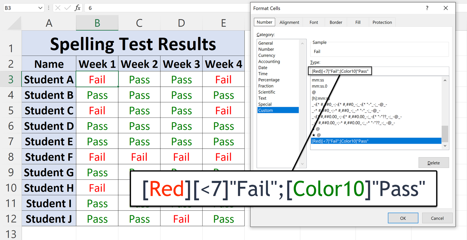
In the late nineties when I was still at primary school, I remember us having a weekly spelling test. There were 10 words the teacher would say aloud, and we would have 30 seconds to write each of them down. The pass threshold was seven marks, and anything below that was deemed a fail.

This was a good way of keeping us on track and an indication of whether we had learnt the words, as we were given prior warning of them.

I have vague recollections of the teacher storing our results on old-fashioned graph paper, as that’s how things were done in those days (unbeknownst to Gen Alpha).

The emphasis was on consistently passing. There was no point in scoring a perfect 10 one week and then getting a drab five the next. It was better just to scrape a solid seven but never drop below.

This nostalgic memory was the inspiration for wanting to show you a quick Excel hack.

You might have a similar scenario, where you want to input a discreet value but display a dichotomous output. Adjusting the cell format allows you to do just that, whilst leaving the underlying value unaffected.

Do the following:

1. Press Ctrl + 1 to open the Format Cells window.
2. In the Number tab, select Custom from the Category list.
3. In the Type field, enter the following:

[Red][<7]”Fail”;[Color10]”Pass”

Values below seven will output as “Fail” (in red) and ones seven or above as “Pass” (in green).

You can use the following named colours:

• [Black]
• [Green]
• [White]
• [Blue]
• [Magenta]
• [Yellow]
• [Cyan]
• [Red]

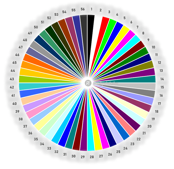
Or you can select one from Excel’s original palette of 56 colours (see image). You don’t, however, have access to the 16.7 million that Excel 2007 and beyond have in the colour window.

Another limitation is you can’t have more than two conditions. However, the key advantage over Conditional Formatting is you can control how the value outputs.