Highlight Row Blocks in Excel

Excel Tables has a Banded Rows option that highlights rows in alternating colours. This enhances readability by making it easier to differentiate between them.

What if you wanted to highlight blocks of rows though?

A conditional formatting rule combining the ISODD/ISEVEN, CEILING and ROW functions can achieve this.

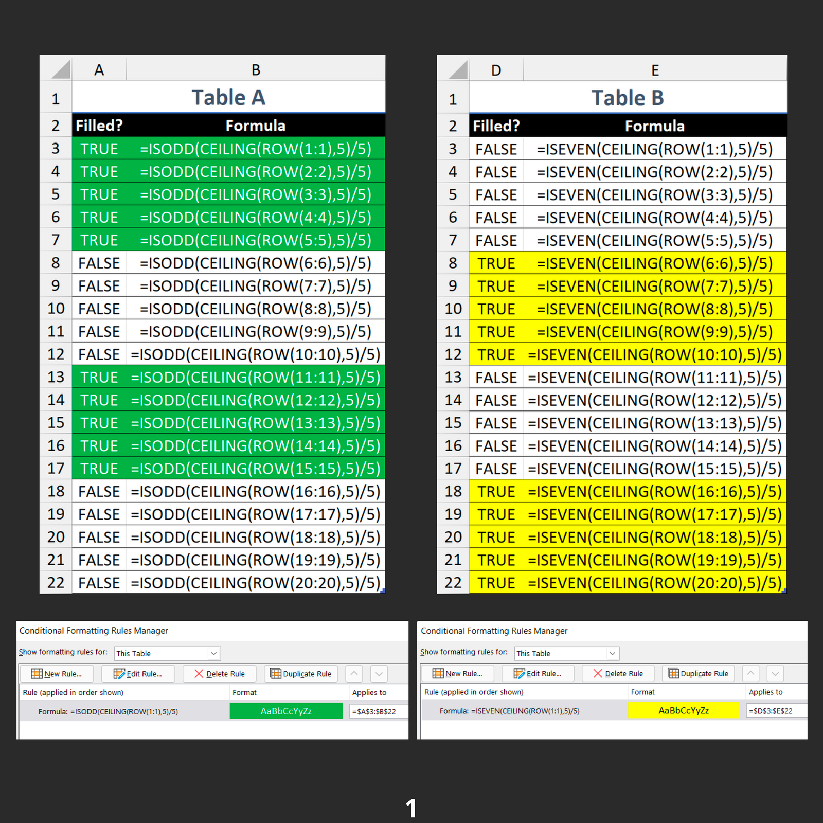
On page 1, a set of TRUE and FALSE values is generated for each table in blocks of five. These determine the cells that should have formatting applied.

The top row formulas (A3 and D3) are put forward as the rules used in the Conditional Formatting window. Each formula adapts to the cells in the applied range.

Let’s break down the Table A example starting in cell A3:

=ISODD(CEILING(ROW(1:1),5)/5)

• ROW(1:1) — returns the row number 1.
• CEILING(ROW(1:1),5) — rounds up 1 to the nearest multiple of 5, which is 5.
• ISODD(CEILING(ROW(1:1),5)/5) — 5 ÷ 5 = 1, so TRUE is returned because 1 is an odd number.

A8 contains the first FALSE entry:

=ISODD(CEILING(ROW(6:6),5)/5)

6 is rounded up to 10, and as 10 ÷ 5 = 2, FALSE is returned because 2 is even.

Table B does the opposite of Table A, as ISEVEN is used to fill the cells that were previously left blank.

Page 2 shows the effect of combining these rules. They are suited to data with a predictable number of records in a block. In this case, regions are banded together so the start and end can easily be seen.