Excel Cell Errors Explained
Staring at a worksheet with a plethora of errors is not sightly, but it can be your saving grace for diagnosing formula problems.
Over a dozen error types exist, and chances are you will have seen most of them at some point, but you wouldn’t necessarily be able to pinpoint when and why they appear.
This article looks in-depth at the types of cell errors and the scenarios that cause them to occur.
Before We Start
Download the complementary workbook here:
Please view in a Windows-based Microsoft 365 desktop version of Excel for maximum compatibility.
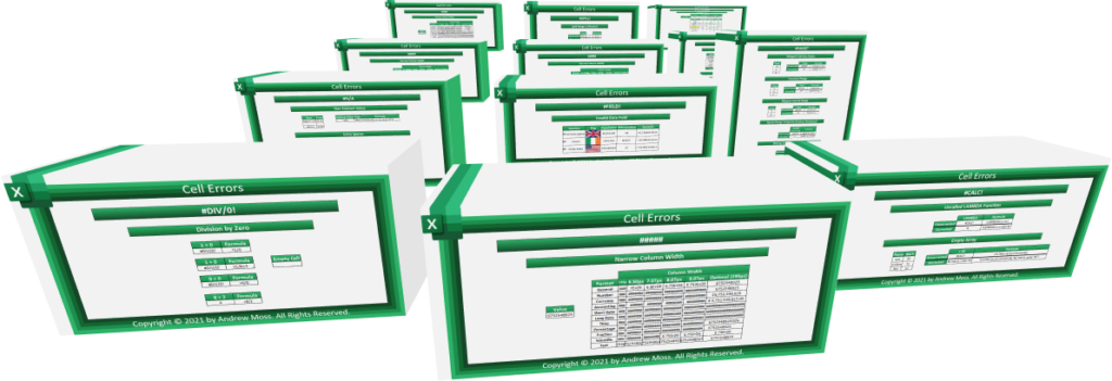
The examples for each cell error are housed in separate worksheets. Use the tabs to navigate between them.

Cell Errors
#####

Cause(s):
Narrow Column Width
This isn’t an error caused by a formula, but if a column’s width is too narrow to display a numeric value, it will result in a set of hash symbols. However, the cell format also determines when they show up.
The General format will make the number display in exponential notation first — with fewer decimal places as the column narrows. For example, 6752548925 becomes 6.753E+09, 6.75E+09, 6.8E+09 and then 7E+09. When the column gets even narrower, the hash symbols appear.
Scientific does the same, except as it defaults to two decimal places, the hash symbols kick in at a later point.
The Number, Currency, Accounting and Percentage formats also default to two decimal places but do not work like this. They either show the whole number or fill the cell with hash symbols if it doesn’t fit.
Text isn’t affected by any of these things and will display what it can regardless of the column width.
#CALC!

Cause(s):
Uncalled LAMBDA Function
When you’re testing out a LAMBDA function, typically you’ll construct it in a cell first before pasting it into Name Manager. Failing to call it by not providing any parameter values will result in a #CALC! error.
Here, x and y are the parameters and x+y is the calculation, but no values have been given for x and y.

The problem is solved when 2 and 6 are fed in as x and y, respectively, allowing the calculation 2+6 to take place.

Empty Array
Any array returned by the FILTER function must consist of at least one row, otherwise, it isn’t valid.
#CALC! appears in cell M18 as there are no marks under 50 in the range J18:J20.

The optional if_empty argument can be used to replace the error with a value of your choice.

#DIV/0!

Cause(s):
Division by Zero
In mathematical terms, a non-zero figure divided by zero produces an undefined result, whilst zero divided by itself is called indeterminate. Excel doesn’t differentiate between these, so #DIV/0! will occur for both.
It’s worth remembering that empty cell references are also considered zeros.
#FIELD!

Cause(s):
Invalid Data Field
Excel fails to retrieve additional information from a cell using a data type because it’s an unknown value.
Any cell can be converted to a data type by going to the Data tab and selecting the appropriate one from the Data Types section.

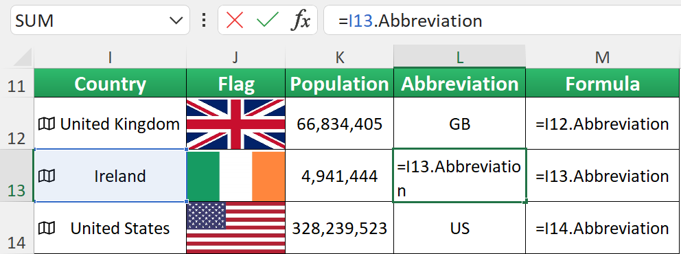
Although Ireland is a recognised geographic entry, it does not have an Abbreviation option like the United Kingdom and the United States. That’s why the formula =J13.Abbreviation returns the #FIELD! error.


#N/A
N/A is a commonly seen initialism that means not available. This gives you a clue what the #N/A error does.
It appears when a lookup formula fails to return a value — and is associated with the XLOOKUP, VLOOKUP, HLOOKUP, INDEX and MATCH functions.
Sometimes a missing value is obvious, but other times it’s caused by obscure things such as extra spaces, misspellings, or incorrect ranges.
Cause(s):
Non-Existent Value
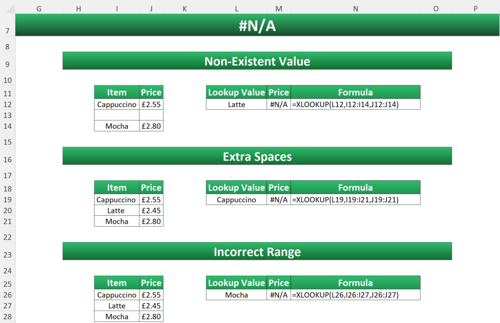
In this XLOOKUP formula, Latte is the coffee name to return the price for, but no such table value exists.

Extra Spaces
There is nothing wrong with the formula here, and it’s easy to be baffled about why it isn’t working. However, the issue lies with the data.

Spaces are invisible and virtually undetectable, especially when they appear at the end of values.
In cell I19, there is a solitary space after the word Cappuccino. It might seem trivial, but this differs from the lookup value in L19, making it impossible to find.

Incorrect Range
The lookup value is Mocha, which appears in the table but isn’t part of the reference in the lookup_array argument— neither is the price for return_array. If just one of these was referenced properly though, a #VALUE! error would be produced instead of #NA.

#NAME?

Cause(s):
Misspelt Function Name
Always ensure you have spelt a function correctly, as it’s easy to double type or omit a character.
The SUM function has been spelt ‘SUMM’, which is non-existent.

Incorrect Range
A range must be consistent on both sides of the colon. For instance, you can’t reference a cell on the left side and only a column on the right.

Misspelt Named Range
A named range must be referenced correctly in the formula, so ensure there are no misspellings.
In cell L26, a non-existent name called Value is included in the SUM formula. If you go to the Formulas tab and click on Name Manager, you’ll see an entry called Values. This was the intended name.

Named Range Scoped to Another Worksheet
Named ranges must have the correct scope to be used in a worksheet.
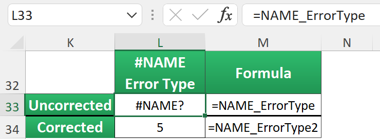
Inside Name Manager, highlight NAME_ErrorType and click on the Edit button; this opens the Edit Name window.

The Scope dropdown determines which worksheet the named range is compatible with. As it’s bound to Error Handling, it will only work in cells there.
Once you have assigned a workbook-wide or worksheet-specific scope and clicked OK, it cannot be changed as the dropdown will be greyed out. You will have to create a new name if you want a different scope. That’s why it’s better to stick to Workbook, like for NAME_ErrorType2.

Missing Quotes in Text Value
A text string must be surrounded by quotation marks, otherwise, it will be interpreted as a name.

Smart Quotes in Text Value
Be careful not to use the wrong type of quotation marks. Only the straight variant will work.

#NULL!
Cause(s):
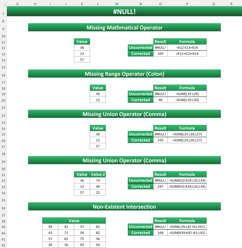
Missing Mathematical Operator
An absent mathematical operator like the plus (+), minus (–), multiply (*), or division (/) symbol will make the calculation incomplete.

Missing Range Operator (Colon)
A colon (:) sandwiched between two cell references is necessary to indicate it is a range.

Missing Union Operator (Comma)
A comma is an argument separator. It’s needed here to separate the [number1] and [number2] SUM arguments.

Non-Existent Intersection
A space character is an intersection operator. If it’s used, the ranges must overlap each other for the calculation to be valid.


#NUM!

Cause(s):
Impossible Calculation
A mathematically impossible calculation will fail to compute and produce a #NUM! error.
√-1 doesn’t work because the square root of any number is always positive (except √0), so the #NUM! error is invoked.

Number Outside Min/Max Boundaries
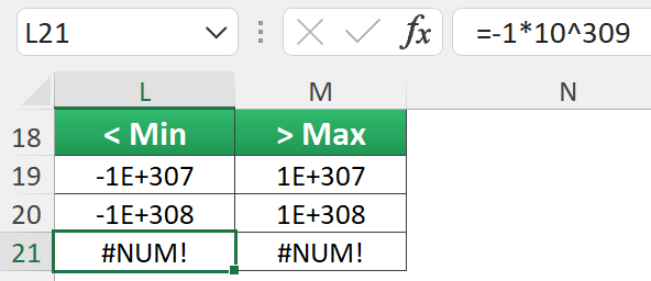
The smallest number possible in Excel is -1*³⁰⁸, whereas the largest is 1*³⁰⁸. That is -1 and 1 both followed by 308 zeros!
Any number outside these boundaries isn’t valid.
End Date Precedes Start Date
DATEDIF is an undocumented function and does not appear in the Insert Function window or IntelliSense. However, if you use it to find the difference between two dates, the end date must not precede the start date.

Iterative Formula Failure
Functions like RATE, IRR, and XIRR use iteration to find a result. Excel restricts the number of iterations, so if a result isn’t found before the limit, a #NUM! error is returned.

The iteration settings can be adjusted by going to File > Options > Formulas > Calculation.
#REF!

Cause(s):
Invalid Reference
An invalid reference will produce a #REF! error. Usually, this happens because sheets, rows or columns have been deleted.
In the example, try deleting rows 12 to 21.
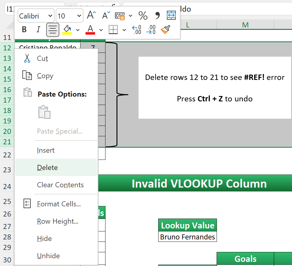
This triggers a #REF! error in J12.

After, press Ctrl + Z to undo and return to the previous state.
Invalid VLOOKUP Column
You will also see a #REF error with the VLOOKUP function when an invalid number is specified in the col_index_num argument.
As there are only two columns in the lookup table, a col_index_num of 3 cannot work.

*TIP*

It’s best to ensure there are no cell references that point to what you’re deleting, so always be cautious. However, if you find any #REF errors, it’s good practice to fix them immediately.

Manually check for them using the Find and Replace window (Ctrl + F or Ctrl + H). You can also replace each instance with a new reference.
#SPILL!

Cause(s):
Spill Range is Blocked
A non-blank cell must not exist in the range the formula is trying to spill in.
As the value 2 exists in cell K12, it prevents the adjacent formula from working.
#VALUE!
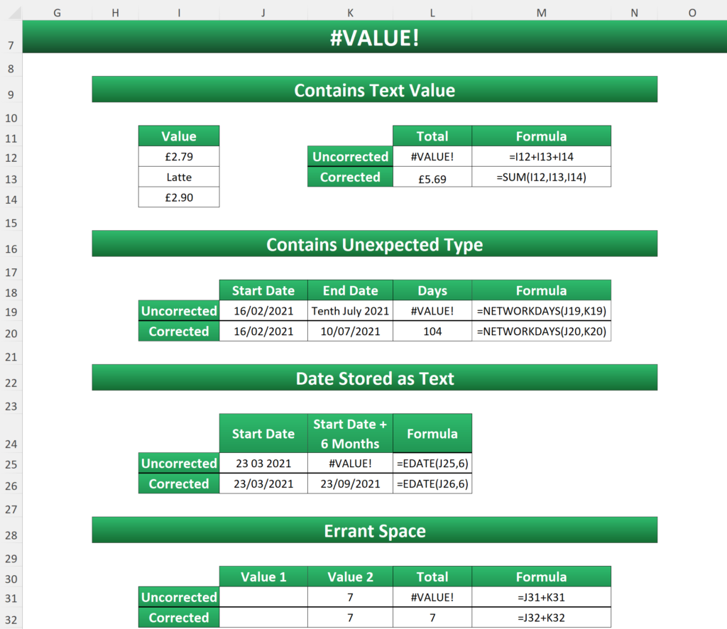
Cause(s):
Contains Text Value
If you add a group of values by summing them individually, there cannot be any text values. However, if you use the SUM function, text values will be ignored.

Contains Unexpected Type
The NETWORKDAYS function requires a start and end date in the correct format. Text is not permitted.

Date Stored as Text
Entering an invalid date format will automatically convert to text, so ensure it is one Excel recognises.

Errant Space
When summing individual cells, be aware of ones that look blank but actually contain a space.

Other Errors
There are also a few other errors that appear less frequently, but let’s quickly run through them:
#BLOCKED!
Returned when a required resource cannot be accessed.
This has been known to appear when attempting to use the STOCKHISTORY function in the free online version of Excel. It won’t work because a Microsoft 365 subscription is required.
#BUSY!
This indicates a formula is fetching a required resource that is taking a long time to access. This might be because:
- an external workbook link contains values a formula is waiting for
- an image is being rendered
- a function is still executing due to a complex calculation or the retrieval of an external resource
⛔ ️#CONNECT!
At the time of writing, no source has documented this error.
#GETTING_DATA
In large, complex worksheets, this will temporarily show up in cells still processing.
#UNKNOWN
Appears when the cell’s assigned data type is not supported in the Excel version you are running.
Error Handling
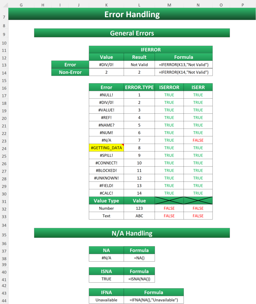
General Errors
There are three functions for general error handling.
IFERROR targets all error types, and the one returned is replaced with a chosen value.
It has two arguments:
value—the value to check for an error.
value_if_error—the value you want to replace the error with.

ISERROR evaluates the value argument and outputs TRUE if it returns an error.
ISERR evaluates the value argument and returns TRUE for all error types except #N/A.
These functions were tested on each error type to clarify what they return.

Trapping every error isn’t always what you’ll want. Sometimes you’ll want to home in on certain ones.
Target a specific error with the ERROR.TYPE function. For example, =IF(ERROR.TYPE(K22)=6,TRUE,FALSE) checks cell K22 for error 6, which equates to #NUM!. As it indeed does, TRUE is returned.
There seems to be a bug associated with the #GETTING_DATA error in K24. If you save the workbook, close it and then reopen it, it changes to #N/A. However, the adjacent ERROR.TYPE remains as 8 until you reconfirm the formula.
N/A Handling

Given the prevalence of #N/A errors, it’s lucky enough to get its own set of functions! There are three:
- NA — returns the value #N/A
- ISNA — returns TRUE if a value is #N/A
- IFNA — returns a specified value if an expression resolves to #N/A
Final Words
There are more error types in Excel than you probably realised! However, the likelihood is you will only encounter a few of them regularly. Still, it’s good to be aware of them as you’ll be able to fix formulas faster.
The IFERROR function is useful for clearing up a worksheet of errors, but try to understand your formulas first so you know what errors are returned and why.
If, for example, you have a lookup formula, the most common error will be #N/A. However, suppressing all the others as well makes it harder to know their cause. That’s why IFNA might be a better choice.
ERROR.TYPE gives you the ultimate flexibility though. Used in conjunction with the AND function, you can target not just one, but multiple error types.
Whatever you use, think carefully about your choices to aid you in creating more efficient formulas.
