Building an Excel football league table — 5 years on

Five years ago (almost to the day), I published my first-ever blog post. It also happened to be on my birthday, funnily enough.
What did I decide to write about?
Well, what better place to start than the very thing that got me into Excel in the first place?
That’s right — football league tables.
There were already numerous sources that had covered how to do this, so I thought: what can I do differently?
I didn’t just want to show you the old-fashioned way of building them, as dynamic arrays had just burst onto the scene. At the same time, I didn’t want to neglect compatibility, as many people were still stuck with dusty old versions of Excel.
Therefore, I was compelled to showcase the old school methods and the new ones. In fact, just look at what I said at the end of that article:
“Hopefully the workbook examples have given you food for thought with how you can go about creating formulas that make use of Excel’s dynamic array powers. The centralised, one formula = many cells approach will gradually become the de facto standard, so get ahead of the curve whilst you can.”
On reflection, saying “gradually” was probably an overstatement. The reality is that in 2025, most Excel users still haven’t caught on or caught up — perhaps they’ve touched the surface at best.
The average office Excel workbook remains inefficient, fragile, and prone to error. That’s because they’re typically bloated with hundreds of tangly formulas, auxiliary tables, helper columns, and a spiderweb of precedents and dependents.
Don’t blame employees entirely for this. A lack of training, standards, and leadership all contribute to poorly built workbooks. Not to mention that many companies are painfully slow to update their versions of Microsoft 365. Some even insist on avoiding subscription fees by clinging to perpetual copies instead, completely oblivious to the enormous benefits of Modern Excel.
Admittedly, larger companies in particular do have to be warier of change, as the cost is likely to be exponentially higher if something messes up.
However, is compatibility on my radar anymore when I’m devising solutions? Absolutely not.
I ain’t going back to the old days. There have simply been too many great features and functions to arrive. Having to cater for older Excel versions just isn’t worth the time and effort anymore.
What has changed in the last 5 years?
Quite a lot. In 2020, it felt like a revolution to have dynamic arrays unleashed upon us alongside functions such as XLOOKUP, SEQUENCE, SORT, and UNIQUE.
However, now our toolbox includes the likes of CHOOSECOLS, HSTACK, VSTACK, IMAGE, LAMBDA, MAKEARRAY, and MAP.
None of these were available back then, thus couldn’t be used. However, their release has expanded the possibilities, allowing us to do some remarkably clever things.
In fact, if you thought what I showed you last time was mightily impressive, what you’re about to see will blow your mind.
Before we proceed
Download the example file: building-an-excel-football-league-table-5-years-on.xlsx
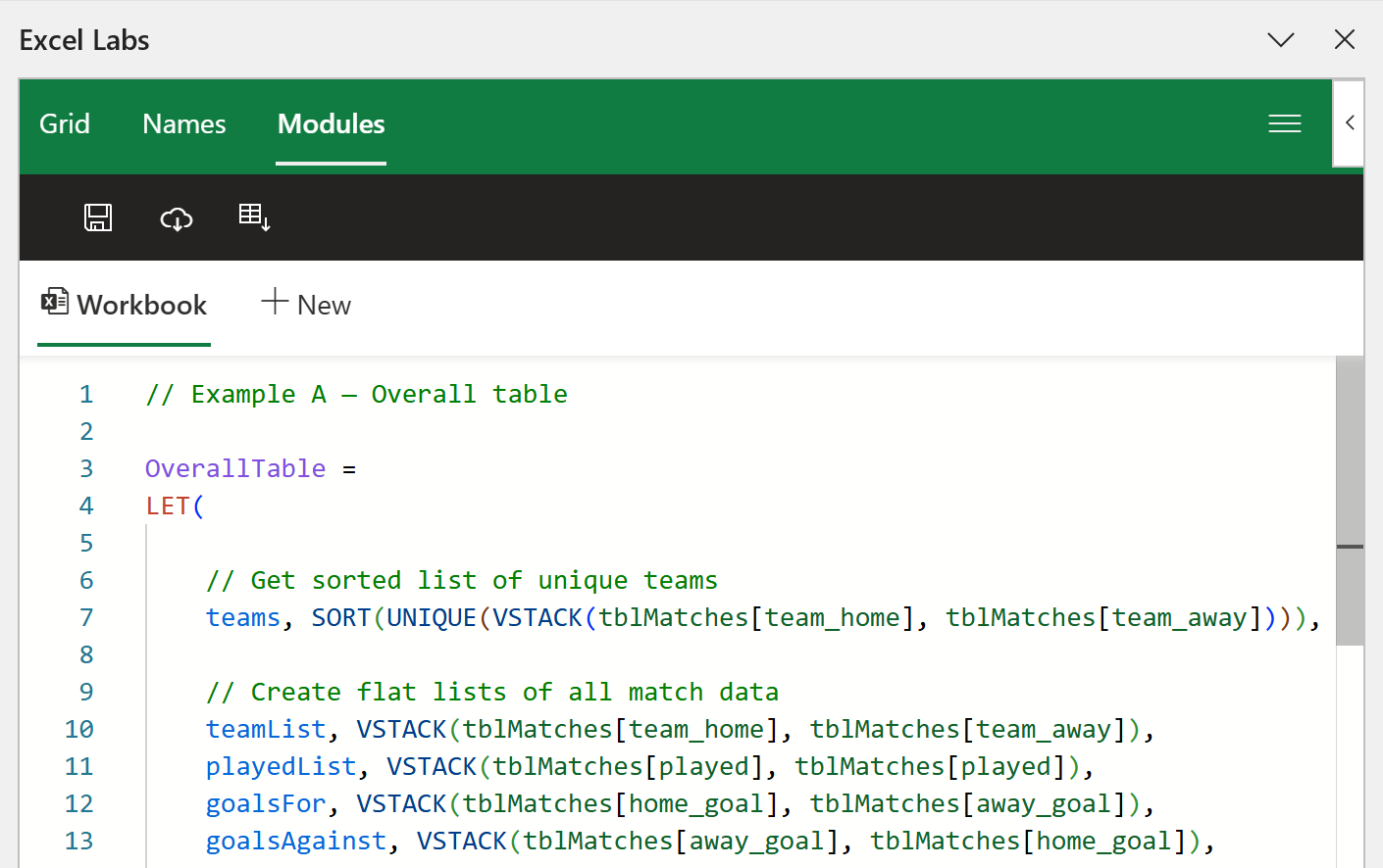
You’ll need Excel for Microsoft 365 to see everything work. Also, ensure you have the Excel Labs add-in installed, as I used the Advanced Formula Environment to write these formulas. The standard formula bar is really not designed for this stuff!
What’s in the workbook?
The workbook contains three worksheets: Data, Example A, and Example B.
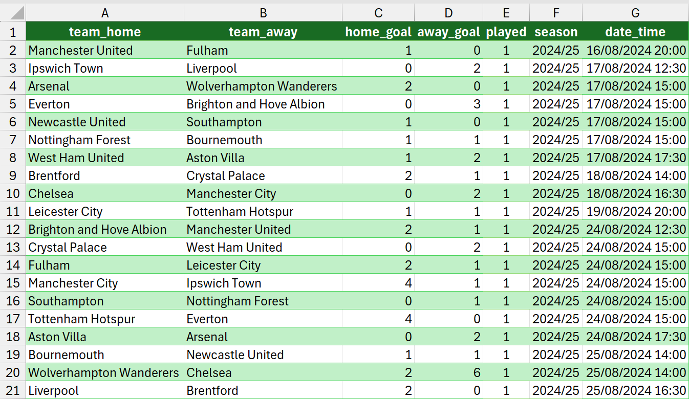
In Data, all 380 matches from the 2024/25 Premier League season are housed in a table called tblMatches.
Adjacent to this is another table called tblTeams, containing all 20 team names alongside their respective crests.
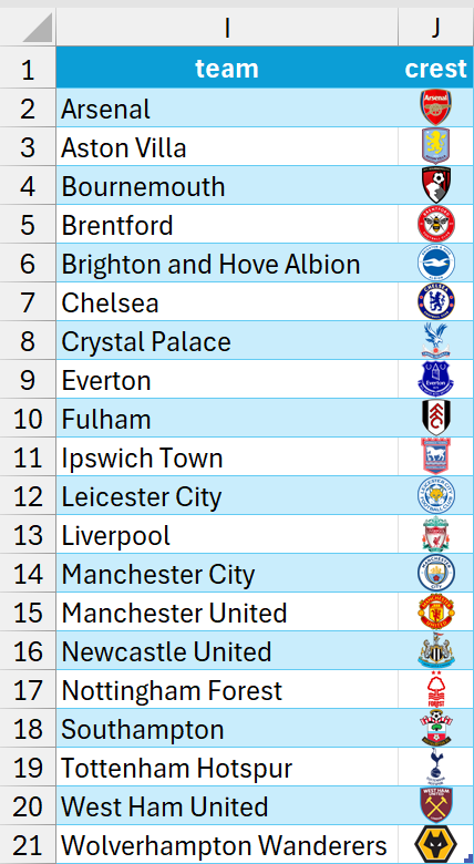
These have been taken from Wikipedia, with a little help from the IMAGE function.
For example, Arsenal’s crest is extracted using =IMAGE("https://upload.wikimedia.org/wikipedia/en/thumb/5/53/Arsenal_FC.svg/1920px-Arsenal_FC.svg.png").
Building the Overall table
Take a quick glance at the Overall table in the Example A worksheet.
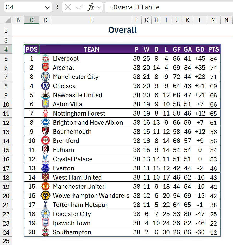
There may be 231 cells involved, but there aren’t the same number of formulas or static values. Last time, the best I got it down to was three formulas, but this uses just one in C4 and spills everything across and down to M24.
It’s the purest form of centralisation I was talking about!
The formula behind =OverallTable in C4 is:
// Example A — Overall table

OverallTable =
LET(

    // Get sorted list of unique teams
    teams, SORT(UNIQUE(VSTACK(tblMatches[team_home], tblMatches[team_away]))),

    // Create flat lists of all match data
    teamList, VSTACK(tblMatches[team_home], tblMatches[team_away]),
    playedList, VSTACK(tblMatches[played], tblMatches[played]),
    goalsFor, VSTACK(tblMatches[home_goal], tblMatches[away_goal]),
    goalsAgainst, VSTACK(tblMatches[away_goal], tblMatches[home_goal]),

    // Calculate metrics per team
    pld, MAP(teams, LAMBDA(team, SUM((teamList=team) * playedList))),
    wins, MAP(teams, LAMBDA(team, SUM((teamList=team) * playedList * (goalsFor>goalsAgainst)))),
    draws, MAP(teams, LAMBDA(team, SUM((teamList=team) * playedList * (goalsFor=goalsAgainst)))),
    gf, MAP(teams, LAMBDA(team, SUM((teamList=team) * playedList * goalsFor))),
    ga, MAP(teams, LAMBDA(team, SUM((teamList=team) * playedList * goalsAgainst))),
    gd, gf - ga,
    losses, pld - wins - draws,
    pts, wins * 3 + draws,

    // Look up crest URLs; empty string remains empty
    crestURLs, MAP(teams, LAMBDA(team,
        IF(team="","",
            XLOOKUP(team, tblTeams[Team], tblTeams[Crest], "")
        )
    )),

    // Assemble raw table: TEAM | CREST | P | W | D | L | GF | GA | GD | PTS
    rawTable, HSTACK(teams, crestURLs, pld, wins, draws, losses, gf, ga, gd, pts),

    // Sort by PTS, GD, GF (ignore crest for sort order)
    sortOrder, {10,9,7},
    sortDir, {-1,-1,-1},
    sortedTable, SORT(rawTable, sortOrder, sortDir),

    // Add position column
    pos, SEQUENCE(ROWS(sortedTable)),

    // Build final table: POS | CREST | Team | P | W | D | L | GF | GA | GD | PTS
    body, HSTACK(
        pos,
        CHOOSECOLS(sortedTable,2),  // CREST
        CHOOSECOLS(sortedTable,1),  // TEAM
        CHOOSECOLS(sortedTable,3,4,5,6,7,8,9,10) // Metrics
    ),

    // Define headers
    headers, {"POS", "", "TEAM", "P", "W", "D", "L", "GF", "GA", "GD", "PTS"},

    // Output headers and body
    VSTACK(headers, body)
)It starts by pulling in all the home and away match data from tblMatches and flattens it into a single list using VSTACK. This makes it much easier to perform calculations.
Next, MAP loops over each team, calculating matches played (P), wins (W), draws (D), losses (L), goals for (GF), and goals against (GA). Goal difference (GD) is simply GF minus GA, and points (PTS) follow the usual standard of three for a win and one for a draw.
Once the stats are in place, the formula looks up each team crest from tblTeams. If no crest is found, an empty string is returned. After that, the team names, crests, and stats are stitched together into a raw table using HSTACK. This is then sorted by points (PTS), goal difference (GD), and then goals scored (GF). The last two are necessary so the table can handle tiebreakers if one or more teams are level on points.
Next, SEQUENCE and ROWS are used to add a position column (POS). CHOOSECOLS then determines the order of the columns to output, before the headers are defined in an array.
The final stage is to use VSTACK to, quite literally, stack the headers on top of the main part of the table.
Building the Home and Away tables
Now that the hardest table is out of the way, let’s move on to the first of the two easier ones.
Unlike the Overall table, this only takes home matches into consideration, rather than away ones as well.
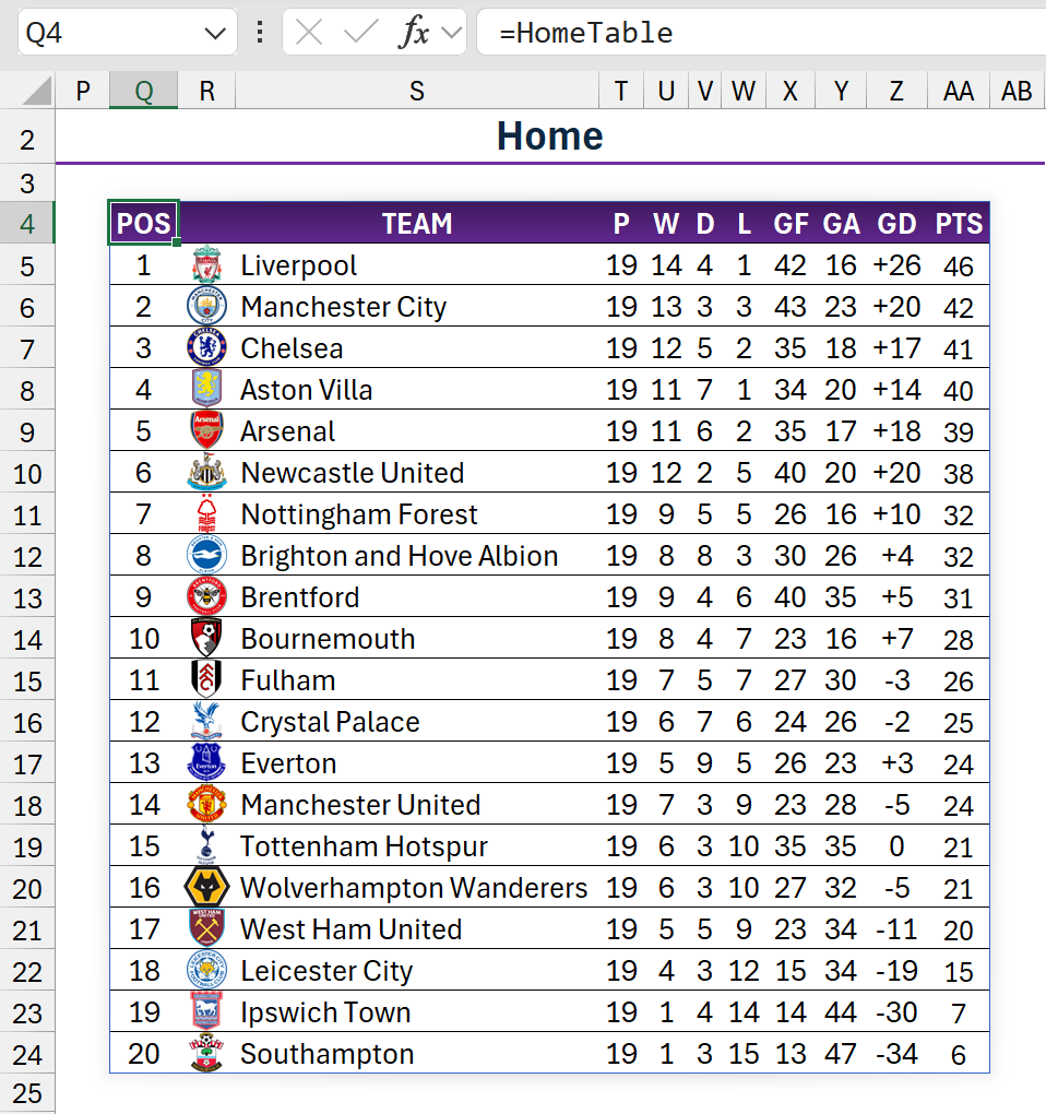
The formula behind =HomeTable in Q4 is:
// Example A — Home table

HomeTable =
LET(

    // Get sorted list of unique teams (from home matches only)
    teams, SORT(UNIQUE(tblMatches[team_home])),

    // Home-only data
    teamList, tblMatches[team_home],
    playedList, tblMatches[played],
    goalsFor, tblMatches[home_goal],
    goalsAgainst, tblMatches[away_goal],

    // Metrics
    pld, MAP(teams, LAMBDA(team, SUM((teamList=team) * playedList))),
    wins, MAP(teams, LAMBDA(team, SUM((teamList=team) * playedList * (goalsFor>goalsAgainst)))),
    draws, MAP(teams, LAMBDA(team, SUM((teamList=team) * playedList * (goalsFor=goalsAgainst)))),
    gf, MAP(teams, LAMBDA(team, SUM((teamList=team) * playedList * goalsFor))),
    ga, MAP(teams, LAMBDA(team, SUM((teamList=team) * playedList * goalsAgainst))),
    gd, gf - ga,
    losses, pld - wins - draws,
    pts, wins * 3 + draws,

    // Look up crest URLs
    crestURLs, MAP(teams, LAMBDA(team,
        IF(team="", "",
            XLOOKUP(team, tblTeams[Team], tblTeams[Crest], "")
        )
    )),

    // Assemble raw table: TEAM | CREST | P | W | D | L | GF | GA | GD | Pts
    rawTable, HSTACK(teams, crestURLs, pld, wins, draws, losses, gf, ga, gd, pts),

    // Sort by PTS, GD, GF
    sortedTable, SORT(rawTable, {10,9,7}, {-1,-1,-1}),
    pos, SEQUENCE(ROWS(sortedTable)),

    // Final table: POS | CREST | TEAM | P | W | D | L | GF | GA | GD | PTS
    body, HSTACK(
        pos,
        CHOOSECOLS(sortedTable,2),  // CREST
        CHOOSECOLS(sortedTable,1),  // TEAM
        CHOOSECOLS(sortedTable,3,4,5,6,7,8,9,10) // Metrics
    ),

    // Headers
    headers, {"POS", "", "TEAM", "P", "W", "D", "L", "GF", "GA", "GD", "PTS"},

    // Output
    VSTACK(headers, body)
)The formula is pretty much the same structurally as the Overall table, with the exception of the column references in certain places aided by VSTACK.
The changes are as follows:
teamsUNIQUE(VSTACK(tblMatches[team_home], tblMatches[team_away]))↓UNIQUE(tblMatches[team_home])
teamListVSTACK(tblMatches[team_home], tblMatches[team_away])↓tblMatches[team_home]
goalsForVSTACK(tblMatches[home_goal], tblMatches[away_goal])↓tblMatches[home_goal]
goalsAgainst
VSTACK(tblMatches[away_goal], tblMatches[home_goal])
↓tblMatches[away_goal]
As you can imagine, the Away table is exactly like the Home one, with predictable changes.
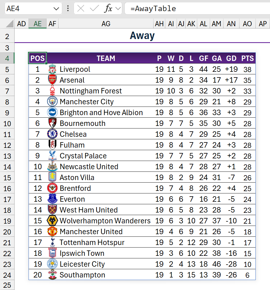
The formula behind =AwayTable in AE4 is:
// Example A — Away table

AwayTable =
LET(

    // Get sorted list of unique teams (from away matches only)
    teams, SORT(UNIQUE(tblMatches[team_away])),

    // Away-only data
    teamList, tblMatches[team_away],
    playedList, tblMatches[played],
    goalsFor, tblMatches[away_goal],
    goalsAgainst, tblMatches[home_goal],

    // Metrics
    pld, MAP(teams, LAMBDA(team, SUM((teamList=team) * playedList))),
    wins, MAP(teams, LAMBDA(team, SUM((teamList=team) * playedList * (goalsFor>goalsAgainst)))),
    draws, MAP(teams, LAMBDA(team, SUM((teamList=team) * playedList * (goalsFor=goalsAgainst)))),
    gf, MAP(teams, LAMBDA(team, SUM((teamList=team) * playedList * goalsFor))),
    ga, MAP(teams, LAMBDA(team, SUM((teamList=team) * playedList * goalsAgainst))),
    gd, gf - ga,
    losses, pld - wins - draws,
    pts, wins * 3 + draws,

    // Look up crest URLs
    crestURLs, MAP(teams, LAMBDA(team,
        IF(team="", "",
            XLOOKUP(team, tblTeams[Team], tblTeams[Crest], "")
        )
    )),

    // Assemble raw table: TEAM | CREST | P | W | D | L | GF | GA | GD | PTS
    rawTable, HSTACK(teams, crestURLs, pld, wins, draws, losses, gf, ga, gd, pts),

    // Sort by PTS, GD, GF
    sortedTable, SORT(rawTable, {10,9,7}, {-1,-1,-1}),
    pos, SEQUENCE(ROWS(sortedTable)),

    // Final table: POS | CREST | TEAM | P | W | D | L | GF | GA | GD | PTS
    body, HSTACK(
        pos,
        CHOOSECOLS(sortedTable,2),  // CREST
        CHOOSECOLS(sortedTable,1),  // TEAM
        CHOOSECOLS(sortedTable,3,4,5,6,7,8,9,10) // Metrics
    ),

    // Headers
    headers, {"POS", "", "TEAM", "P", "W", "D", "L", "GF", "GA", "GD", "PTS"},

    // Output
    VSTACK(headers, body)
)The changes are:
teamsUNIQUE(tblMatches[team_home])↓UNIQUE(tblMatches[team_away])
teamListtblMatches[team_home]↓tblMatches[team_away]
goalsFortblMatches[home_goal]↓tblMatches[away_goal]
goalsAgainst
tblMatches[away_goal]tblMatches[home_goal]
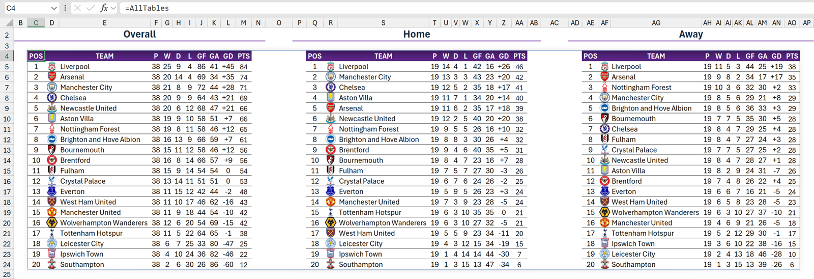
Stacking the tables
In Example A, there were three tables, each built with a single formula, despite the total real estate spanning 693 cells.
Example B takes things to the next level by joining the Overall, Home, and Away tables, so only one formula is required to display all three.
It’s pretty easy to do!
The formula behind =AllTables in C4 is:
// Example B — all tables

AllTables =
LET(
    gap, MAKEARRAY(ROWS(OverallTable), 3, LAMBDA(r,c,"")),
    HSTACK(
        OverallTable,
        gap,
        HomeTable,
        gap,
        AwayTable
    )
)Key to this is MAKEARRAY, which is used to include three columns between each table. This statement is assigned to the LET named value gap and then referenced inside HSTACK between the named formulas.
What you’ve just seen is modular design in a nutshell. It’s about treating your components like reusable Lego blocks.OverallTable, HomeTable, and AwayTable are individual units that can be combined, reused, or repurposed depending on your needs.
If you want to tweak one, you can do so without affecting any of the others. Although it’s certainly possible, there’s always a greater risk everything will break if all three complete formulas are squeezed into one, which is why it’s generally better to build them separately and then stack them later.
Formatting the tables
To make the tables look pretty in both worksheets, I spruced them up with a bit of colour and borders. Unfortunately, though, this involves a separate process.
You can either use the standard ribbon formatting options to do this or rely on Excel’s incredibly archaic conditional formatting system.
I chose the latter.
Two rules were created for each table — the purple one for the headers and the other for the body. The purpose is to check if the first cell in the range isn’t empty using ISBLANK.
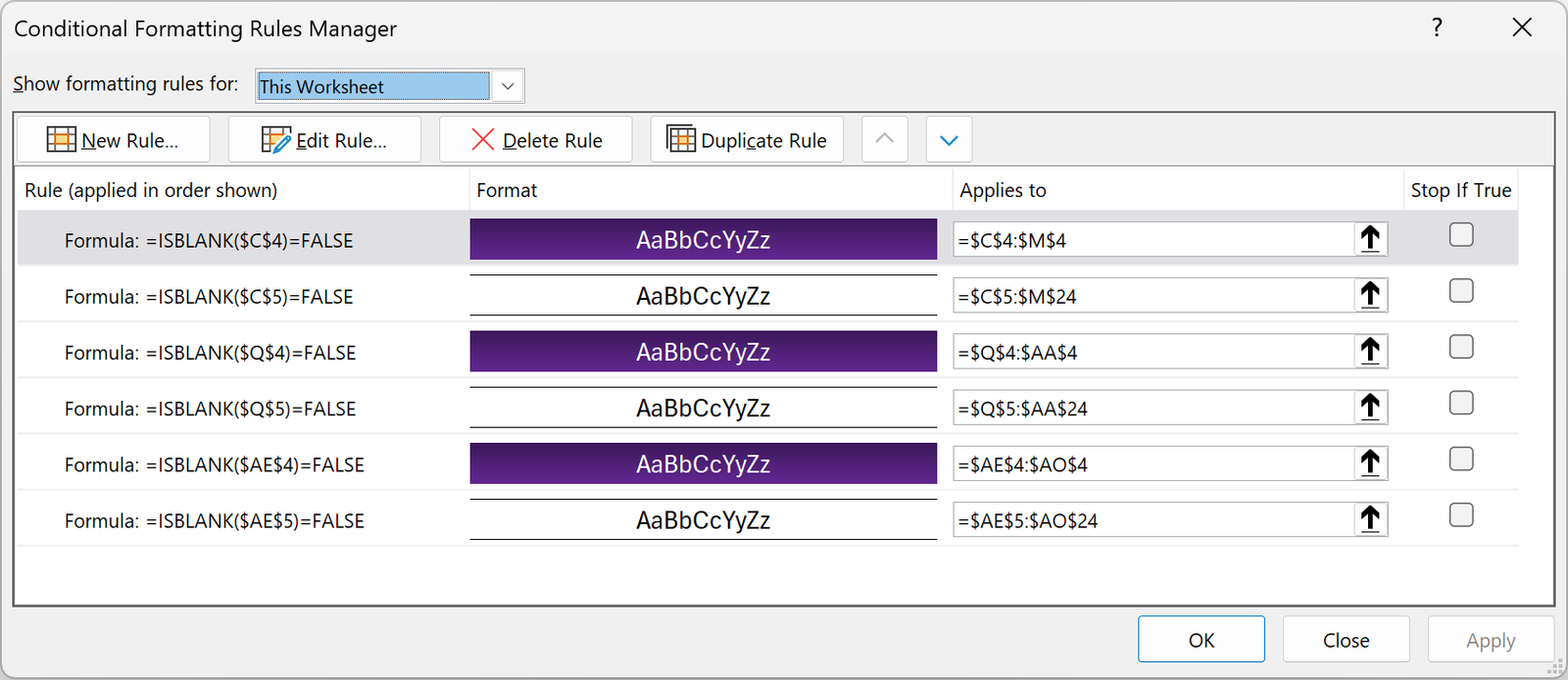
For all the bad things, that’s the one good thing about conditional formatting. It can be made to switch on and off depending on whether the formula name exists in the cell. For example, if =OverallTable is present in C4, the formatting displays. If not, everything is blank in C4:M24.
You know what irks me, though? When you build these impressive dynamic array formulas, it highlights inadequacies elsewhere. The current formatting and conditional formatting systems certainly fall into that bracket.
What we need is the ability to manipulate these in the formula language, so they can be an integrated part of a calculation. I’m talking about having, for example, a FORMAT function that gives us all the major ribbon formatting options. Perhaps it could be combined with IF for conditional formatting.
As a basic example, would something like the following suffice?

// Header formatting

LET(
    headers, {"POS", "", "TEAM", "P", "W", "D", "L", "GF", "GA", "GD", "PTS"},
    formattedHeaders, FORMAT(headers,
        {"background.color", "font.bold", "font.color"},
        {"purple", TRUE, "white"}
    ),
    formattedHeaders
)I know you’ve heard the term a lot in recent years, but that really would be a game-changer.
Conclusion
The last five years have been an exciting time for Excel, with so many exciting updates rolled out to us.
Having said that, it has died down over the past 18 months due to the emergence of Copilot, which Microsoft seemingly wants to impose on every aspect of our workflow.
Nevertheless, hopefully you can take these concepts and apply them to your own work. While the formulas I showed you might look intimidating at first, adapting to this approach is the way forward.
Think about that report you’ve built — the one that’s propped up by a plethora of helper columns, intermediary formulas, and auxiliary tables.
Now imagine stripping all of that away and replacing it with a clean, centralised, and modular formula system built in the Advanced Formula Environment.
You’ll bulletproof your workbooks and make them easier to maintain and debug.
Admittedly, taking dynamic arrays to the extreme won’t always be appropriate for your scenario. But you should at least make it a habit to think: how can I do this better?
Once you realise there’s a better way, you’ll wonder why you didn’t discover it sooner.


